博客

  • Troubleshooting Mass Flow Meter Error Codes in Daily Operations

    Troubleshooting Coriolis Mass Flow Meter Error Codes in Daily Operations
    Coriolis • Field Troubleshooting Guide

    Troubleshooting Coriolis Mass Flow Meter Error Codes in Daily Operations

    A field-technician-focused guide to the error codes you’ll actually see. Organized by what’s failing — sensor, signal, process, or electronics — with a decision tree for fast triage and concrete steps you can take before calling support.

    A Coriolis meter that’s throwing an error code is not always a broken meter. In many field investigations, the meter is working correctly and the error is telling you something about the process — entrained gas, a drifting zero, an installation stress that changed last week. Distinguishing “the meter is sick” from “the meter is healthy but its job has gotten harder” is the main skill of Coriolis troubleshooting, and it’s the main skill this guide is built around.

    Coriolis error code systems differ by manufacturer in their naming and numbering, but the underlying failure categories are the same across brands. This guide uses generic category names (like “Drive Gain High” or “Tube Not Oscillating”) and cross-references the typical equivalents in Emerson Micro Motion, Endress+Hauser Promass, KROHNE OPTIMASS, and similar lines — so the workflow is portable across whatever meter is actually on the skid.

    The structure is built for the way a field technician actually works: a decision tree for fast triage, followed by detailed problem cards for the error classes you’ll encounter most. Use the tree first to narrow down which category of error you’re looking at, then jump to the card that matches. Each card is self-contained — you don’t need to read the whole guide to solve one error.

    01 — Before You Touch

    Triage Principles Before You Touch Anything

    The most expensive troubleshooting mistakes happen in the first five minutes — usually as a well-intentioned “let me just reset the meter and see.” Four principles reduce the chance of making a diagnosable problem into an undiagnosable one.

    Principle 1

    Read the error before clearing it

    Many error codes are latched — they’re telling you that a condition occurred, even if the condition has passed. Clearing the error without logging the code, the timestamp, and the recent process trends destroys information you may need ten minutes later when the same error returns. Always document before you reset.

    Principle 2

    Correlate with the process, not just the meter

    A density drift alarm that appeared at the same moment as a feed composition change is telling you about the process. A drive gain alarm that appeared with no process change is telling you about the meter or its installation. The first question is always “what else changed around this time?” — not “what’s wrong with the meter?”

    Principle 3

    Distinguish continuous from intermittent

    A continuous error usually points at a hardware or installation issue (failed pickoff, loose connection, chronic installation stress). An intermittent error usually points at a process condition (transient two-phase flow, pulsation at startup, pump cycling). The fix is different; confusing the two leads to replacing hardware that wasn’t the problem.

    Principle 4

    Check the easy things first, always

    Wiring connections at the terminal block, grounding, transmitter power supply, and recent maintenance activity account for a large share of “sensor failure” calls. Five minutes of checking the terminal box beats two hours of advanced diagnostic menus. The hierarchy is: connections → installation → process → sensor → electronics.

    The meter is the suspect only after the wiring, the installation, and the process have been cleared.
    02 — The Vocabulary

    Error Code Naming Across Brands

    Every Coriolis manufacturer uses a different code format. Emerson Micro Motion uses alphanumeric codes (A003, A104, A131). Endress+Hauser Promass uses S-codes and F-codes (S144, F274). KROHNE OPTIMASS uses four-digit numerics. The underlying error conditions, however, map to a small number of generic categories that are identical across vendors — because the physics being diagnosed is identical.

    This guide uses generic category names throughout, because a field technician working on mixed-brand sites is better served by understanding the failure mode than by memorizing one vendor’s code list. Each error card in Sections 4–7 cross-references the generic name to the typical equivalents in the major brands. Exact code numbers should always be verified against the specific meter’s operating manual — vendor firmware revisions occasionally shift codes between versions.

    CATEGORY 01
    Sensor
    Pickoff failure, coil continuity, RTD failure, tube not oscillating
    CATEGORY 02
    Signal
    4–20 mA output, HART/Modbus comm loss, signal saturation
    CATEGORY 03
    Process
    Two-phase flow, high drive gain, zero drift, density out of range
    CATEGORY 04
    Electronics
    Transmitter memory error, internal voltage fault, firmware integrity

    In a typical field population, process-category errors are by far the most common (60–75% of alarms on most sites), followed by sensor-category errors (15–25%), then signal and electronics (the remainder combined). The proportions justify where this guide spends its detail — sensor and process errors are expanded in depth; signal and electronics are kept compact.

    03 — The Map

    The Field Decision Tree

    Start here when an error is active. The tree routes from the top-level symptom (“is the meter reading anything at all?”) down to the error category, then to the specific card. If you arrive at a leaf node and the remedy doesn’t apply, back up one branch and reconsider the previous answer.

    Coriolis Error Triage — Field Decision Tree START error code shown on HMI Q1 · Is the transmitter powered and displaying any value? NO Electronics § 7 YES Q2 · Is the tube oscillating? (check drive gain / freq in diagnostics) NO Sensor § 4 · Tube Not Oscillating YES Q3 · Does a 4–20 mA meter at the terminals show live data? NO Signal § 6 YES Q4 · Is drive gain > 40% or noise/variance elevated? YES Process § 5 · Drive Gain High NO Q5 · At zero flow, does the reading drift away from zero? YES Process § 5 · Zero Drift NO Q6 · Does density reading match the known fluid density? NO Process § 5 · Density Out of Range YES Subtle sensor issue — pickoff asymmetry or RTD fault likely — LEGEND — yes path hardware process
    Start at the top node. At each question, follow the Yes or No branch. Terminal nodes route to the detailed error card in Sections 4–7. The tree assumes you’ve already completed the triage checks from Section 1 (wiring, power, recent changes).
    04 — Category One

    Sensor-Category Errors — Detailed

    Sensor-category errors indicate a problem in the physical measurement chain — flow tubes, drive coil, pickoff sensors, or the integrated RTD. These errors are typically continuous rather than intermittent and usually require physical inspection or replacement. They are less common than process errors, but more consequential when they occur.

    Sensor CRITICAL

    Tube Not Oscillating

    Emerson ≈ A003·Endress ≈ F274 / F276·KROHNE ≈ Sensor Fault
    What the Meter Is Telling You

    The drive circuit is active but the pickoff sensors are not detecting tube motion within the expected frequency band. Mass flow and density outputs are frozen at zero or held at the last valid value, depending on fail-safe configuration.

    Most Likely Causes (in order)

    1. Tubes empty or partially filled. The meter was taken out of service and the tubes drained; now the drive coil can excite the tubes but the natural frequency is shifted so far outside the expected range that the pickoff detection logic rejects it. Most common cause on a “new error after maintenance” call.

    2. Drive coil circuit open or shorted. Check with a multimeter at the transmitter terminals — the drive coil typically reads a few hundred ohms; open circuit or dead-short is a broken coil or a cable fault.

    3. Pickoff sensor failure. Less common than drive coil failure. Both pickoffs failing simultaneously is rare; one pickoff failed usually produces a “tube imbalance” error instead, not “not oscillating.”

    Field Check Sequence
    1. Confirm the tubes are full. Check the upstream block valve position; verify process line is not drained. If the meter is new and just commissioned, confirm the purge or fill procedure was completed.
    2. Measure drive coil resistance. Transmitter OFF, disconnect drive leads, measure with a multimeter. Value should match the meter datasheet (typically 100–400 Ω depending on model). Open, short, or wildly off-spec = coil fault.
    3. Measure pickoff coil resistance. Same procedure on the two pickoff leads. Both should read within ~10% of each other.
    4. Check cabling continuity. If the meter electronics are remote-mounted, pickoff and drive signals travel through a field cable — inspect connectors and verify continuity at the meter end.
    Resolution

    If tubes are empty → refill line and retry. If coil fault confirmed → sensor is not field-repairable; schedule replacement. If cabling fault → replace or reterminate cable.

    Time to resolution: 15 min (empty tubes) to multi-day (sensor replacement requiring shutdown).
    Sensor WARNING

    Tube Imbalance / Sensor Asymmetry

    Emerson ≈ A104·Endress ≈ S156·KROHNE ≈ Asymmetric Signal
    What the Meter Is Telling You

    The two pickoff sensors are producing signals of different amplitudes — typically beyond a vendor-defined tolerance of 10–20%. The meter can still compute mass flow but the internal balance that underlies zero stability is compromised.

    Most Likely Causes

    1. One pickoff degraded. Internal coil aging, slight winding degradation, or connector contact resistance drift. The asymmetry often develops gradually over years.

    2. Tube coating (uneven). On heavy hydrocarbons, waxy process fluids, or biofilm-prone services, uneven coating on one tube shifts its effective mass relative to the other.

    3. Installation stress. Piping stress that deforms one tube’s mounting more than the other — usually appears after recent piping work nearby.

    Field Check Sequence
    1. Record pickoff amplitudes from diagnostics menu. Note the ratio. If ~1:1, error is spurious; if >1.2:1, asymmetry is real.
    2. Check recent maintenance history. Any piping modifications upstream or downstream in the last 90 days? Recent shutdown with a refill procedure?
    3. Consider fluid cleaning. If service is known-fouling, a mild flush (per vendor recommendation) may restore balance.
    4. Measure pickoff coil resistances. If resistances differ significantly, one pickoff has degraded.
    Resolution

    Cleaning resolves most coating-induced asymmetry. Installation-stress cases require piping correction. Genuine pickoff degradation is non-field-repairable and requires sensor replacement — though many meters will continue to run with degraded accuracy for extended periods if the asymmetry is stable.

    Sensor WARNING

    RTD Fault / Temperature Sensor Out of Range

    Emerson ≈ A017 / A018·Endress ≈ F041 / F043·KROHNE ≈ RTD Fail
    What the Meter Is Telling You

    The integrated RTD (used for temperature compensation of mass flow and density) is reading outside its valid range, typically <−50 °C or >+200 °C, or showing an open-circuit or shorted condition. Mass flow and density continue to update but without proper temperature compensation — accuracy degrades.

    Most Likely Causes

    1. RTD wiring fault. Loose terminal, water ingress in junction box, or field-cable issue on remote-mount installations.

    2. RTD element failure. Rare — Pt100 elements are typically very reliable, but mechanical shock or extreme thermal cycling can fail one.

    3. Genuine out-of-range process condition. Startup from ambient where line was not yet at operating temperature; or a process upset creating unusually cold or hot conditions.

    Field Check Sequence
    1. Check the reported temperature. If it’s exactly the minimum or maximum of range, likely an electrical fault. If it’s a plausible process value, likely a configuration or range issue.
    2. Verify RTD wiring. Transmitter OFF, check wiring continuity and insulation resistance.
    3. Cross-check with an adjacent temperature measurement. Any nearby TT on the same line that should read approximately the same value?
    Resolution

    Wiring fix or RTD replacement (vendor service). Until resolved, document the impact on measurement accuracy and notify process operations — density accuracy is particularly sensitive to RTD loss.

    05 — Category Two

    Process-Category Errors — Detailed

    Process-category errors are the most frequent class of Coriolis alarms in field operations. They indicate that the measurement conditions have changed — not that the meter has failed. Resolving them usually means diagnosing an upstream process change, not servicing the meter. Getting this right is where field-technician experience pays off most.

    Process WARNING

    Drive Gain High / Drive Saturation

    Emerson ≈ A102 / A131·Endress ≈ S144 / S145·KROHNE ≈ High Drive
    What the Meter Is Telling You

    The drive circuit is applying more energy than usual (often >40% of max) to maintain tube oscillation. The tubes are being damped by something that wasn’t there during calibration — almost always entrained gas, particulates, or a tube-coating change.

    Most Likely Causes (in order)

    1. Two-phase flow — entrained gas in liquid or liquid slugs in gas. By far the most common cause. Can be transient (startup, pump priming) or continuous (degassing from dissolved gas, flashing on pressure drops).

    2. Solids content. Slurry service, particulates in produced fluids, or crystallization on a cooling line. Tubes are fine but the fluid is more lossy than calibration.

    3. Tube damage. Erosion, cracking, or a stuck valve near the sensor. Usually associated with a step change in drive gain, not a gradual drift.

    Field Check Sequence
    1. Check density reading. If density is wildly different from expected (particularly: dropping below fluid density on liquid service) → entrained gas is confirmed, skip to (4).
    2. Check process stability. Is the drive gain transient (spiking at pump starts, settling) or continuous? Transient = operational; continuous = sustained condition.
    3. Check upstream pressure. If pressure dropped recently, dissolved gas may be flashing out. Common cause on cryogenic or hydrocarbon service.
    4. Confirm two-phase with a density trend. Density jitter or a sawtooth pattern over time = two-phase flow.
    Resolution

    Transient two-phase: usually operational — tolerate during startup, ensure meter is after the pump with adequate back-pressure for steady-state. Continuous two-phase: add a degasser upstream, raise line pressure, or accept accuracy limitations during the affected conditions. Slurry/particulates: meter may be correctly operating — verify accuracy spec covers this service. Tube damage: replace.

    Remember: “Drive gain high” is usually not a hardware problem. 80%+ of drive gain alarms on process plants trace to two-phase flow or a related process condition.
    Process WARNING

    Zero Stability Error / Zero Drift

    Emerson ≈ A008 / A017·Endress ≈ S147·KROHNE ≈ Zero Shift
    What the Meter Is Telling You

    At no-flow conditions, the meter is reading a non-zero value. The zero offset has drifted from its last calibrated value, or the meter is showing a zero value during no-flow that doesn’t match the stored zero point.

    Most Likely Causes

    1. Zero was calibrated under different conditions than current service. Zero must be established at the actual operating temperature, pressure, and full-flooded state — not during commissioning at ambient with an empty line.

    2. Installation stress changed. Piping movement from thermal expansion or recent work shifted stress on the meter body. This can cause a persistent apparent zero offset that a new zero calibration will correct.

    3. Real flow during the “zero” check. Block valves not fully sealed, a drain or bypass leaking, or a slow backflow — the meter is correctly reading a small flow.

    Field Check Sequence
    1. Confirm genuinely no-flow conditions. Both upstream and downstream block valves closed and confirmed tight. No bypasses, no drains open.
    2. Check if tubes are full. Empty or partially-filled tubes produce false zero readings.
    3. Check temperature stability. Zero calibration is only valid at the temperature it was performed at; major temperature shifts require re-zeroing.
    4. Perform a new zero calibration per vendor procedure. Only after the above are confirmed.
    Resolution

    In nearly all cases: re-zero under correct conditions (full, stable, no-flow, at operating temperature). If re-zero doesn’t hold, investigate installation stress — that points to a piping support or alignment issue rather than a meter issue.

    Process INFORMATIONAL

    Density Out of Range / Unusual Density

    Emerson ≈ A033·Endress ≈ M801·KROHNE ≈ Density Warn
    What the Meter Is Telling You

    The measured density is outside the expected range configured in the transmitter. The meter is not failing — it’s producing a reading that doesn’t match configured expectations. Often a service composition change, sometimes a two-phase indicator.

    Most Likely Causes

    1. Actual composition change. Different grade of crude, concentration shift in a chemical recipe, or a product changeover not reflected in transmitter configuration.

    2. Two-phase flow pulling density down. Entrained gas lowers apparent density below the pure-liquid value; usually accompanies a drive gain alarm.

    3. Temperature compensation error. If RTD is reading wrong (see RTD fault card), density compensation will be wrong too.

    Field Check

    Compare density reading to the expected fluid density at operating temperature. If materially lower than pure-fluid value, suspect two-phase. If materially different but stable, suspect composition change. If tracking temperature incorrectly, suspect RTD. A lab sample can confirm composition.

    Resolution

    Update transmitter density range configuration if the new composition is operational; address two-phase per the drive gain card; repair RTD if temperature-compensation fault.

    Process INFORMATIONAL

    Flow Rate Out of Range / Saturation

    Emerson ≈ A140·Endress ≈ S443·KROHNE ≈ Flow Hi/Lo
    What the Meter Is Telling You

    Flow rate has exceeded the configured upper limit (saturation) or has fallen below the lower cutoff. The meter is still measuring, but the output channel may be clamped or flagged as out-of-spec.

    Resolution

    Usually a sizing or configuration issue rather than a meter fault. Verify the meter is correctly sized for the operating range, update the configuration if the process has shifted operating point, or flag the event to process operations if it indicates a genuine upset.

    06 — Category Three

    Signal-Category Errors

    Signal-category errors indicate problems in the output chain between the transmitter and the receiving system — 4–20 mA loops, HART digital communication, Modbus, or Foundation Fieldbus. The measurement itself may be healthy; only the transport is failing. These errors resolve at the wiring or receiving-system level, not at the meter electronics.

    Signal WARNING

    4–20 mA Loop Fault / Output Saturation

    Emerson ≈ A113·Endress ≈ F829·KROHNE ≈ Current Out Fail
    What the Meter Is Telling You

    The 4–20 mA output cannot drive its expected current — either a loop break (open circuit) or saturation at 20+ mA (short or too low resistance). The transmitter is trying to send a signal that the wiring will not accept.

    Quick Checks

    Verify loop resistance (typically 250–600 Ω depending on installation), check continuity of the 2-wire cable, verify the receiving device (PLC analog input, DCS card) is powered and configured. Loop breaks often trace to loose screw terminals after maintenance activity.

    Resolution

    Correct the wiring fault, replace a damaged cable segment, or reconfigure the receiving device. The meter itself usually does not require attention.

    Signal INFORMATIONAL

    Digital Communication Loss / HART or Modbus Fault

    typically not shown on meter; detected at receiving side
    What the Meter Is Telling You

    The DCS or host system has lost digital communication with the transmitter. The meter may still be reading correctly locally, and the 4–20 mA signal may still be working — only the digital overlay (HART) or replacement (Modbus, Fieldbus) has stopped.

    Quick Checks

    For HART: verify loop resistance is within HART tolerance (250 Ω minimum), check for nearby EMI sources, confirm handheld can connect locally. For Modbus/Fieldbus: verify address, baud rate, termination resistors, and segment topology.

    Resolution

    Communication issues rarely trace to meter hardware — look at wiring, termination, host-system configuration, and segment topology first. Field DTM / EDDL software updates on the host side are a common culprit after system upgrades.

    07 — Category Four

    Electronics-Category Errors

    Electronics-category errors indicate a fault in the transmitter itself — memory corruption, internal voltage regulation, or firmware integrity. These are uncommon in field populations (well under 5% of total alarms on most sites) and are rarely user-repairable. The response is typically escalation to the manufacturer, not field repair.

    Electronics CRITICAL

    Electronics Fault / Memory or Voltage Error

    Emerson ≈ A001 / A002·Endress ≈ F270 / F271·KROHNE ≈ Electronics Fail
    What the Meter Is Telling You

    The transmitter’s self-diagnostics have detected an internal fault — bad checksum on configuration memory, internal voltage out of range, or failed startup self-test. Measurement outputs may be frozen, held at failsafe, or absent.

    Quick Checks

    Verify supply voltage is within meter specification (typically 18–30 VDC for 4-wire meters); check for water ingress in the transmitter housing; check for recent power events (lightning, surge, interrupted commissioning).

    Resolution

    Power-cycle may clear transient faults. Persistent electronics faults should be escalated to the vendor — these are not user-serviceable. A transmitter swap (with configuration restore from backup) is usually the only field-applicable remedy.

    Electronics WARNING

    Configuration Error / Corrupt Configuration

    Emerson ≈ A027 / A029·Endress ≈ C410·KROHNE ≈ Config Fault
    What the Meter Is Telling You

    The transmitter’s configuration data (meter constants, calibration factors, fluid properties) has failed a self-integrity check, or a configuration write was interrupted. Often appears after a firmware upgrade or after recent HMI activity.

    Resolution

    Restore configuration from the vendor’s backup file (every properly commissioned meter should have a configuration backup). If no backup exists, the meter requires re-commissioning with original calibration data obtained from the vendor — this is why backups matter.

    08 — The Reference

    Quick-Reference Error Table

    Print this page and keep it near the HMI. A 30-second scan should point to the right detailed card in sections 4–7.

    At-a-Glance Error Reference
    Generic Error Name Category Severity First Check Likely Root
    Tube Not OscillatingSensorCriticalTubes full?Empty line / coil fault
    Tube ImbalanceSensorWarningPickoff amplitudesCoating / stress / aging
    RTD FaultSensorWarningTemperature reading valueWiring / RTD failure
    Drive Gain HighProcessWarningDensity reading stable?Two-phase flow
    Zero DriftProcessWarningGenuinely no-flow?Zero calibration stale
    Density Out of RangeProcessInfoKnown composition?Composition or 2-phase
    Flow SaturationProcessInfoSizing vs actualConfig or process upset
    4–20 mA Loop FaultSignalWarningLoop continuityWiring issue
    HART/Modbus Comm LossSignalInfoLocal vs hostHost or segment issue
    Electronics FaultElectronicsCriticalSupply voltage / moistureTransmitter hardware
    Configuration ErrorElectronicsWarningRecent HMI activity?Interrupted write
    09 — The Prevention

    Prevention & Routine Checks

    The errors above are easier to prevent than to fix. A short monthly routine and a longer annual routine catch the majority of developing issues before they become alarms.

    Monthly — 10 minutes per meter

    Record drive gain, pickoff amplitudes, density at steady flow, and zero reading. Compare to previous months. Trending beats absolute values — a drive gain rising from 12% to 22% over six months is a story, even if 22% is still below the alarm threshold.

    Quarterly — density cross-check

    Pull a lab sample from a port near the meter. Compare lab density (temperature-corrected) to meter density reading. A gap >1 kg/m³ developing over time often indicates tube coating — address before the drive gain alarm activates.

    Annually — zero calibration under correct conditions

    Re-zero the meter under process temperature and pressure, with tubes confirmed full and flow confirmed to be zero. Document the zero value. A zero that drifts more than the vendor spec year-over-year indicates an installation issue developing.

    Always — keep a configuration backup

    Every commissioning, every firmware upgrade, every significant configuration change — back up the transmitter configuration and label it with date and reason. The “Configuration Error” alarm card depends on this: a backup turns a major problem into a 10-minute restore.

    10 — The Stop

    Escalation Path — When to Stop DIY

    Not every error is a field-fix. Knowing when to stop troubleshooting and call support saves time and avoids making things worse. Three rules bound the DIY zone:

    Rule 1

    Stop after two verified replacements

    If you’ve already replaced the transmitter or the sensor and the same error persists, the problem is not where you’ve been looking. Further replacement attempts are expensive guesses. Call vendor support with your diagnostic data.

    Rule 2

    Stop before opening a sealed sensor

    Coriolis flow tubes and their housings are sealed at the factory. Opening them in the field voids warranty, breaks the hermetic protection against moisture and dust, and — on hazardous-service meters — may invalidate explosion-protection certification. If a sensor needs to be opened, it’s going back to the vendor.

    Rule 3

    Stop if a safety-function meter is involved

    Meters that are part of a SIF (safety instrumented function) or an overpressure protection layer have specific qualification requirements. Any repair or recalibration needs to follow the site’s management-of-change procedure, and the work may need to be vendor-performed to preserve the SIL certification.
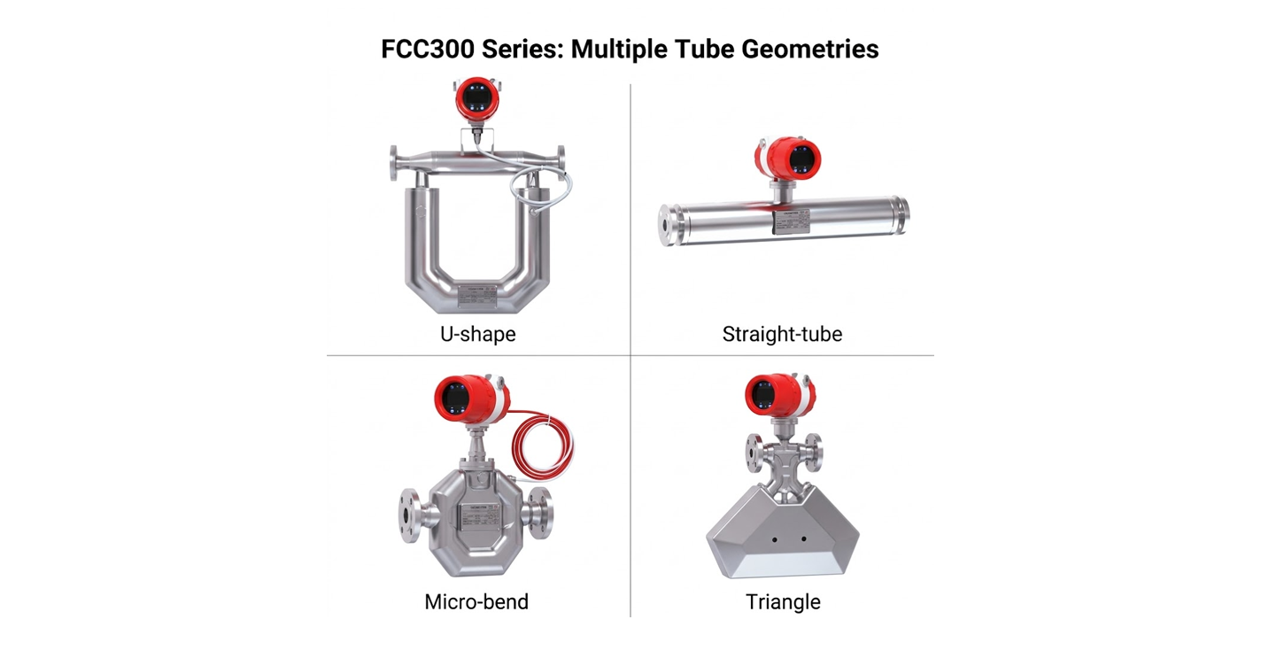
    11 — Product Fit

    Supmea Product Fit

    Supmea’s Coriolis mass flow meter range implements the diagnostic categories described in this guide — sensor, signal, process, and electronics — with error codes that map to the generic naming used throughout. The transmitter provides drive gain, pickoff amplitudes, density, and temperature as diagnostic values accessible from both the local HMI and the HART/Modbus interface, enabling the monthly-and-quarterly verification routine from Section 9 without requiring specialized software.

    For sites running mixed-brand Coriolis populations, Supmea meters fit into the same workflow — field technicians trained on Emerson or Endress meters can apply the same triage sequence and decision tree to Supmea installations. Full product specifications, including complete error-code references, are available on the Supmea product site. For projects specifying new Coriolis installations, the Supmea application team can review diagnostic requirements, alarm configurations, and maintenance workflow before commissioning — so the meters arrive aligned with the site’s existing troubleshooting practice.

    For background on the underlying principles referenced in this guide, external references on mass flow meters and the HART protocol are useful starting points.

    Still Seeing the Error After This Guide?

    Share the error code, the meter model, the measurement context, and what you’ve already checked. Our application team helps narrow down whether you’re looking at a meter issue, an installation issue, or a process change — and what the next concrete step should be.

    Consult Supmea →

    © 2026 Supmea. All rights reserved.  ·  Field Troubleshooting Guide — Coriolis Mass Flow Meter Error Codes

  • How Coriolis Mass Flow Meters Measure Density and Why It Matters

    How Coriolis Mass Flow Meters Measure Density — And Why It Matters
    Coriolis • Technical Guide • Density

    How Coriolis Mass Flow Meters Measure Density — And Why It Matters

    The density reading from a Coriolis meter is not a by-product of mass flow measurement — it’s an independent, high-accuracy measurement that derives value differently in every industry. This guide walks through the principle, the accuracy factors, and the application scenarios where density is the reason you bought the meter.

    Most Coriolis meter specifications list density accuracy as a secondary line item — ±0.5 kg/m³ or ±1 kg/m³ — next to the more prominent mass flow accuracy figure. That placement understates what density actually does inside a plant. In many installations, the density channel is the justification for choosing Coriolis in the first place: a °API figure that enables crude oil custody transfer, a Brix reading that controls a sugar line, a concentration measurement that closes a chemical recipe loop.

    The physical principle is clean. The flow tubes inside a Coriolis meter oscillate at a natural frequency that depends on their own mass plus the mass of fluid inside them. Denser fluid means more mass means a lower frequency. The meter measures this frequency continuously and converts it to density using a calibrated curve. The conversion is direct — no secondary instrument, no inference, no external loop.

    What’s less clean is the set of conditions under which that reading holds its accuracy. Temperature shifts the tube stiffness. Pressure shifts the tube geometry. Entrained gas shifts the effective density. Pipe stress, mounting changes, and even coating build-up shift the baseline. A Coriolis density reading that is perfect on day one can drift 1–2 kg/m³ by year three if those conditions are not managed. This guide walks through both sides — what the density measurement is, and what it takes to keep it worth trusting.

    01 — The Physics

    The Frequency-to-Density Principle

    A Coriolis meter consists of one or two thin-walled tubes, bent into a U, triangular, or straight configuration. A driver coil excites the tubes into mechanical oscillation at their natural frequency. Two pickoff sensors detect the resulting motion at different points along the tubes.

    For mass flow measurement, the meter reads the phase difference between the two pickoffs — proportional to mass flow rate. For density measurement, the meter reads the frequency itself — which depends on the total vibrating mass. Fluid inside the tube contributes to that mass directly, so denser fluid lowers the natural frequency.

    The underlying relationship follows classical mechanics: the tubes behave as a mass-on-spring system. The natural frequency is inversely proportional to the square root of the vibrating mass, and the vibrating mass is the tube mass plus the fluid mass. Working through the algebra and grouping the geometry-dependent terms into calibration constants yields the practical form used in commercial meters:

    Density — Working Form
    ρ = K1 · T2K2
    ρfluid density [kg/m³]
    Tmeasured tube oscillation period (T = 1/f) [s]
    K1, K2calibration constants derived from two reference fluids

    The same relationship is often stated as a proportionality for quick intuition — the square of the period (or equivalently, 1/f²) varies linearly with density:

    Proportionality — Quick Intuition
    T2  ∝  ρ   ⇔   f−2  ∝  ρ
    lower frequency → denser fluid
    higher frequency → lighter fluid (or gas)

    Two points follow from this structure that matter later in the guide. First, because density is read from a frequency — a time-domain measurement — it is inherently more stable than amplitude-based measurements and less affected by electronic drift. Second, because the conversion depends on calibration constants tied to the physical tube, anything that changes the tube’s mechanical properties (temperature, stress, coating, corrosion) shifts the density reading. Those two facts frame the whole accuracy discussion.

    Natural Frequency Shifts with Fluid Density LIGHT FLUID ρ = 700 kg/m³ f ≈ 100 Hz higher frequency WATER ρ = 1000 kg/m³ f ≈ 85 Hz reference DENSE FLUID ρ = 1400 kg/m³ f ≈ 72 Hz lower frequency density increases frequency decreases (as 1/√ρ) Illustrative only — actual frequencies depend on tube geometry and size
    The same flow tube oscillates at a different natural frequency depending on what fluid fills it. The frequency shift is the density signal.
    02 — The Calibration

    Calibration and the Two-Point Method

    The calibration constants K₁ and K₂ are not derived from tube dimensions — they are determined empirically at the factory. The standard procedure is a two-point calibration: the meter’s oscillation period is measured with the tubes filled with two known reference fluids, almost universally air and water at stable temperature. Two equations, two unknowns — K₁ and K₂ are solved and stored in the transmitter.

    This two-point scheme is why modern Coriolis meters can achieve density accuracy around ±0.5 kg/m³ without customer-side calibration. The air-water span brackets most industrial fluids (roughly 1.2 to 1000 kg/m³), and the linear relationship between T² and ρ means interpolation within that span is geometrically sound.

    Where the factory calibration stops being sufficient is in services where higher-than-default accuracy is needed, typically for custody transfer or fiscal measurement. In those cases a site verification or a third reference point (with a reference fluid close to the expected process density) is used to tighten the working accuracy. This is the distinction between “density-capable” meters and “density-certified” meters — and it is worth asking vendors to be specific about at the bid phase.

    Calibration Quality Is Traceable

    Factory density calibration traceability should be available on request — typically documented against national measurement standards (NIST, PTB, or equivalent). For any application where the density reading will be used for trade, tax, or quality control above ±0.5 kg/m³ tolerance, traceability documentation is not optional.

    03 — Scenario One

    Scenario — Oil & Gas Custody Transfer

    Oil & Gas

    Crude Oil, Refined Products, and Pipeline Custody Transfer

    °API measurement · volumetric-to-standard conversion · fiscal reconciliation

    Oil trading happens in standard volume — barrels at 60°F, cubic meters at 15°C. But metered volume at the pipeline inlet is at whatever the line temperature and pressure happen to be. Converting measured volume to standard volume requires knowing the density at metering conditions, and the industry’s universal way of expressing that density is °API gravity.

    A Coriolis meter on a custody transfer station measures mass flow directly and density directly. From density, the meter calculates °API using the API 11.1 correlation, and from density plus temperature, it calculates the volume correction factor (VCF) per API MPMS Chapter 11. The output is standard-volume flow — the number that appears on the custody transfer ticket.

    • Fiscal weight A 0.1 °API error on a 50,000 bbl/day pipeline translates to roughly 25 bbl/day of volumetric disagreement — enough to fail a monthly reconciliation.
    • Crude identification Density distinguishes crude streams commingled in common pipelines; sudden density shifts flag interface passages and slate changes.
    • Quality pricing Crude prices differ by density grade (light sweet vs. heavy sour) by several dollars per barrel; the meter’s density reading feeds the pricing mechanism directly.
    • Line balance Pipeline shrinkage and expansion accounting depends on standard volume reconciliation at entry and exit points — Coriolis density is the reference at both ends.
    Fiscal / Custody Transfer Service

    Accuracy: ±0.3 kg/m³ or better (tighter than factory default, typically via field verification). Repeatability: ±0.1 kg/m³. Temperature compensation: active, using integrated RTD. Pressure compensation: required for high-pressure lines (>40 bar). Traceability: NIST-traceable calibration certificate included with meter.

    Density drift from coating build-up

    Heavy crude and waxy intermediates build up a thin film on the inner tube wall over time. The film adds apparent mass and shifts the density reading upward by 0.5–2 kg/m³ — a drift that looks like a crude slate change and can pass normal diagnostic checks. Scheduled in-situ density verification against a reference (pycnometer sample or prover) is the standard guard.

    Entrained gas on suction-side metering

    Meters installed on the suction side of transfer pumps can see entrained gas during priming and upset conditions. Gas inclusion lowers the apparent density dramatically — it looks like a crude quality change but is an installation artifact. Discharge-side metering with adequate back-pressure is the standard mitigation.

    04 — Scenario Two

    Scenario — Food & Beverage Brix and CIP

    Food & Beverage

    Sugar Concentration, Milk Solids, Juice Blending, and Interface Detection

    Brix measurement · product-to-product changeovers · CIP interface detection

    In food and beverage, density is rarely reported as density. It’s reported as °Brix (sugar concentration), degrees Plato (brewing), total solids (dairy), or simply as the concentration of the primary dissolved species. The Coriolis meter measures density; the transmitter converts density to the product-specific concentration unit using a calibrated table or polynomial.

    The distinguishing feature of food and beverage applications is that the density reading often serves a control function — it’s not just a measurement, it’s a signal that drives a valve, triggers a changeover, or closes a batch. Continuous in-line density measurement replaces the older practice of pulled samples to a refractometer or laboratory hydrometer, which reduces cycle time and eliminates a class of quality escapes.

    • Sugar syrup blending Continuous Brix measurement on a blending header controls dilution water valves in real time. Reduces off-spec syrup from hours per changeover to minutes.
    • Juice concentration Evaporator outlet °Brix drives feed rate control. In-line density replaces hourly sample laboratory turnaround.
    • Milk standardization Density combined with cream or skim addition controls butterfat specification to label tolerance.
    • CIP interface detection During product-to-cleaning-solution and cleaning-to-product transitions, the density drops from product to water; the density derivative signals the interface passage.
    Hygienic / Process Control Service

    Accuracy: ±0.5 to ±1.0 kg/m³ (standard factory calibration usually sufficient). Repeatability: ±0.1 kg/m³ (matters more than absolute accuracy for control loops). Response time: <1 second for CIP interface detection. Hygienic rating: 3-A or EHEDG certification, clamp connections, drainable orientation. Sanitary finish: Ra ≤ 0.8 µm internal surface.

    Two-phase flow during startup

    Air pockets during tank filling or line priming cause transient density drops that look like cleaning-solution passage. The control system may trigger a false changeover and waste product. Meters should be specified with bubble-handling diagnostics, and installations should allow full flooding before density signals are used for control.

    Temperature compensation mismatch

    Brix tables are defined at 20°C. Process lines often run at 40–80°C (heated syrups, concentrated products). The Coriolis meter must apply temperature compensation back to reference conditions before the Brix conversion is applied; otherwise the Brix output is systematically wrong. This is a configuration issue, not a meter issue — but it is frequently miscommissioned.

    05 — Scenario Three

    Scenario — Chemical Concentration Control

    Chemical

    Acid Concentration, Solution Blending, and Reactor Feed Consistency

    Binary concentration · feed blending · batch-to-batch repeatability

    In chemical processing, many streams are binary mixtures — one solute in one solvent, where the density is a monotonic function of composition. Sulfuric acid in water, caustic soda in water, hydrogen peroxide in water, ammonia in water — all of these have well-characterized density-concentration relationships that allow a density measurement to read out directly as a concentration.

    For multi-component or reactive streams, density alone is not sufficient to resolve composition, but it is often still used as a consistency indicator — a way to verify that a reactor feed or a product stream is not drifting from its normal composition band. In this role, density measurement serves batch-to-batch quality assurance rather than real-time composition inference.

    • Acid / base concentration Sulfuric acid concentration for pickling lines, neutralization, and battery acid production — continuous Coriolis density replaces sampling loops.
    • Blending to recipe Solvent dilution, reagent preparation, and solution make-up use density feedback to close the loop on additive valves.
    • Reactor feed verification Continuous density of the feed stream flags deviations from batch recipe, catching formulation errors before they consume reactor charge.
    • Effluent monitoring Density of process effluents provides a gross composition check for compliance and downstream unit protection.
    Process Chemical Service

    Accuracy: ±0.5 kg/m³ (acceptable for most concentration controls, where 0.5 kg/m³ ≈ 0.05–0.1 wt% for typical aqueous solutions). Wetted materials: Hastelloy C-22 / C-276 or Tantalum for aggressive acids; 316L may not suffice. Temperature compensation: critical — concentration-density curves are strongly temperature-dependent. Pressure compensation: typically required only on gas or high-pressure service.

    Tube corrosion shifts the calibration

    Even slight internal corrosion of the flow tube alters the tube mass and stiffness, shifting K₁ and K₂. Density readings drift without any process change. On services where the tube material is marginally compatible (for example, 316L on dilute sulfuric), this shows up as a slow, unexplained density drift over months. Correct material specification is the prevention; periodic density verification against a lab sample is the detection.

    Non-linear density-concentration regions

    Sulfuric acid density is monotonic up to ~98 wt% and then reverses. For fuming or high-concentration acids, the concentration-density correlation has to be applied carefully — a single Coriolis reading can correspond to two concentrations, and the control system needs additional logic (temperature, expected range) to disambiguate. This is a chemistry issue that constrains where density-based concentration control is applicable.

    06 — The Accuracy

    What Actually Affects Density Accuracy

    Across all three scenarios above, the same physical factors drive the gap between nameplate density accuracy and field density accuracy. Understanding which factors dominate in a given service determines whether the factory calibration is sufficient or field verification is needed.

    FACTOR 01

    Fluid Temperature

    Tube stiffness changes with temperature, affecting the natural frequency independently of density. All modern meters compensate using an integrated RTD, but compensation accuracy degrades outside the calibrated range.

    Impact: 0.5–5 kg/m³ if uncompensated
    FACTOR 02

    Process Pressure

    Pressure changes the tube’s effective geometry slightly — a second-order effect on density. Negligible below ~10 bar; significant on high-pressure gas or liquid service.

    Impact: 0.1–1 kg/m³ per 10 bar
    FACTOR 03

    Mounting Stress

    Stress from misaligned piping or temperature-induced growth shifts tube stiffness and therefore density calibration. Installation-quality dependent; typically constant once installed.

    Impact: 0.5–2 kg/m³ systematic shift
    FACTOR 04

    Entrained Gas / Two-Phase

    Even small gas voids dramatically lower apparent density. Modern meters detect and alarm the condition, but the underlying reading is biased whenever two-phase flow is present.

    Impact: 10+ kg/m³ possible
    FACTOR 05

    Coating / Fouling

    Wax, scale, or biofilm build-up on the tube wall adds apparent mass. Progressive drift over months; not detectable from the density reading alone.

    Impact: 0.5–5 kg/m³ progressive
    FACTOR 06

    Erosion / Corrosion

    Loss of tube wall mass from erosion shifts the calibration in the opposite direction of coating. Slow progression; preventable through correct material selection.

    Impact: 0.5–3 kg/m³ progressive
    FACTOR 07

    External Vibration

    Vibration at or near the drive frequency couples into the density signal. Usually filtered digitally, but severe cases (near-matching resonance) produce noise or bias.

    Impact: variable; noise-dominated
    FACTOR 08

    Flow Rate Effects

    At very high flow, the Coriolis force itself slightly affects the vibration pattern. Higher-end meters correct for this; budget meters may show flow-rate-dependent density bias.

    Impact: 0.1–0.5 kg/m³ at high flow

    For most installations, temperature compensation is automatic, pressure compensation is handled through configuration, and the remaining factors fall into one of two categories: installation-time factors (mounting stress, material compatibility, vibration environment) that are decided at design and don’t change, and service-life factors (coating, erosion, corrosion) that drift over operational time and need a verification regime.

    A density reading is only as stable as the tube it’s measured from. Protect the tube, and the reading holds.
    07 — The Map

    Specification Matrix by Application Class

    The three scenarios above can be summarized in a specification matrix that ties application class to the density-related requirements actually needed. This is the table to print out when writing an RFQ.

    Density Specification by Application Class
    Application Class Accuracy Target Repeatability Compensation Verification
    Fiscal / Custody Transfer±0.3 kg/m³±0.1 kg/m³Temp + PressureTraceable cert + field prover
    Process Concentration Control±0.5 kg/m³±0.1 kg/m³Temp (always)Factory cert + periodic sample
    Blending & Recipe±0.5 to ±1.0 kg/m³±0.2 kg/m³Temp (always)Factory cert sufficient
    CIP Interface / Quality Flag±1.0 kg/m³±0.2 kg/m³Temp (always)Factory cert sufficient
    Consistency Monitoring±1.0 kg/m³±0.2 kg/m³Temp (always)Factory cert sufficient
    General Mass Flow + Density±1.0 kg/m³±0.5 kg/m³Temp (always)Factory cert sufficient

    Two observations worth flagging. First, repeatability matters more than absolute accuracy for most control applications — a meter that reads consistently 1 kg/m³ high is easier to live with than one that reads within ±0.3 kg/m³ but varies unpredictably. Specify repeatability explicitly; don’t assume a tight accuracy number implies tight repeatability. Second, the jump from “factory cert sufficient” to “traceable cert + field prover” is a significant cost step — roughly doubling the installed cost of the meter on some configurations. Reserve it for applications where the accounting or regulatory context actually requires it.

    08 — The Warnings

    Common Specification Pitfalls

    Five recurring pitfalls show up in density-application specifications. Each is easy to avoid at the specification stage and expensive to remediate after commissioning.

    Confusing accuracy with repeatability

    Vendor datasheets list both numbers, but buyers often read only one. For control applications, repeatability is the number that matters; for fiscal applications, accuracy is the number that matters. Specify both, and verify which one the vendor’s published number refers to.

    Specifying tight density accuracy without traceability

    A ±0.3 kg/m³ accuracy claim is only meaningful if the calibration is traceable. A meter calibrated against an in-house reference with unknown pedigree can hit any number the vendor chooses. Request the calibration certificate format during bid evaluation.

    Ignoring the temperature compensation range

    Meters are typically calibrated across a specific temperature range — often −40 to +100 °C or similar. Operating outside the calibrated range invalidates the accuracy spec, even if the transmitter still produces a reading. Cryogenic service, high-temperature service, and wide-swing services all need explicit compensation-range verification.

    Assuming density accuracy independent of mass flow accuracy

    The two specs come from the same physical measurement. A meter that is sized too large for the service (oversized for low flow) may meet density accuracy at zero flow but degrade at turndown. Meter sizing based on mass flow range should include a check that the density accuracy holds at the low end.

    Skipping the two-phase flow question

    Service that is “normally liquid only” often has gas ingress during startup, shutdown, pump priming, or upset conditions. A density reading during those periods is not wrong in the meter sense — it’s correctly reflecting the two-phase mixture — but it’s wrong for any control or accounting use. Specify how the meter should handle the two-phase condition: alarm, hold last good value, or report honestly and let the DCS filter.

    09 — The Summary

    Pre-Specification Checklist

    A single-page verification list for the bid and commissioning phases. If every item can be answered with evidence, the density reading will deliver its specified accuracy. If three or more cannot, the specification carries foreseeable risk that should be addressed before meter selection.

    Before RFQ

    What the application actually needs

    Application class identified — fiscal, control, blending, or monitoring. Accuracy target documented — as a number, not as “high”. Repeatability target documented — separately from accuracy. Temperature range specified — including startup, upset, and shutdown cases. Pressure range specified — for meters running above 10 bar or on compressible service.

    During Vendor Evaluation

    What the meter specification must include

    Density calibration traceability — NIST, PTB, or equivalent. Calibration temperature range — matches or exceeds operating range. Pressure compensation — enabled and documented for high-pressure service. Two-phase flow handling — alarm behavior documented. Material compatibility certificate — ensures the tube won’t corrode or erode through the service life.

    During Commissioning

    What to verify before handoff

    Temperature compensation active — confirmed by reading density at two different temperatures with same fluid. Zero calibration performed under process conditions — not shipped-as-is. Installation stress checked — piping supports take no meter reaction, meter takes no piping reaction. Baseline density recorded — reference for future drift detection.

    10 — Product Fit

    Supmea Product Fit

    Supmea’s Coriolis mass flow meter range provides density measurement as a standard channel alongside mass flow, with specification levels that align to the application classes described in this guide. The standard factory density calibration meets the ±0.5 to ±1.0 kg/m³ accuracy class appropriate for concentration control, blending, and quality monitoring applications — which covers the majority of food & beverage and chemical use cases.

    For fiscal and custody transfer applications requiring ±0.3 kg/m³ or tighter, Supmea offers enhanced calibration variants with NIST-traceable documentation and support for field verification using reference fluids or provers. The meter range supports the wetted materials discussed in the chemical scenario (Hastelloy C-22 / C-276 for aggressive services), the hygienic certifications discussed in the food & beverage scenario (3-A, EHEDG), and the pressure ratings required for oil & gas pipeline service.

    For project teams specifying a Coriolis meter where density is a primary measurement, the Supmea application team reviews the full context — service fluid, operating temperature and pressure range, target concentration or °API output, verification regime — and recommends the meter class, calibration option, and installation configuration that matches the accuracy the application actually needs. Full product specifications are available on the Supmea product site.

    For background on the principles referenced in this guide, external references on mass flow meters, API gravity, and the Brix scale are useful starting points.

    Specifying Density Accuracy from a Coriolis Meter?

    Share the application class, target accuracy and repeatability, the operating temperature and pressure range, and the verification regime you plan to run. Our application team will recommend the meter class, calibration option, and installation configuration that holds its accuracy through the service life.

    Consult Supmea →

    © 2026 Supmea. All rights reserved.  ·  Technical Guide — Coriolis Density Measurement

  • Best Practices for Mass Flow Meter Impulse-Free Piping Layouts

    Best Practices for Mass Flow Meter Impulse-Free Piping Layouts — Installation Guide
    Mass Flow Meter • Installation Guide

    Best Practices for Mass Flow Meter Impulse-Free Piping Layouts

    Pulsating flow is the most common — and most under-budgeted — source of mass flow meter error. This guide walks through impulse-free layout rules for each meter type, with a DP contrast case, focused on what actually puts project budgets and meter lifetimes at risk.

    A mass flow meter that reads 3% high isn’t obviously broken. The spec sheet accuracy looks fine. The transmitter reports no alarm. The meter lasts a full warranty period. And yet, at the end of the year, the mass balance doesn’t close — and the loss shows up on the wrong line of the P&L.

    A large share of those silent errors trace back to one root cause: pulsating flow arriving at a meter that was sized and installed as if the flow were steady. Reciprocating pumps, piston compressors, pressure regulators cycling against capacity, control valves hunting around setpoint — all of these inject pressure and velocity pulsations into the line. Every meter technology responds to pulsation, but each responds differently.

    This guide walks through impulse-free piping layout best practices for Coriolis, thermal, ultrasonic, and vortex mass flow meters — plus a deliberate contrast with differential-pressure (DP / orifice) metering, because the impulse-line dependency of DP is the easiest way to see why “impulse-free” is a valuable property in the first place. The framing throughout is the procurement and project-management view: what happens to measurement accuracy, to installation rework, and to meter lifetime when pulsation is under-specified.

    01 — The Framing

    Why Pulsation Destroys Measurement Quietly

    Every mass flow meter infers mass flow from some physical proxy — tube vibration phase shift, heat transfer rate, transit-time difference, vortex shedding frequency, or differential pressure across a restriction. When the flow is steady, the proxy is stable and the inferred mass flow is accurate. When the flow is pulsating, the proxy fluctuates — and the averaging logic inside the transmitter almost always introduces bias.

    The critical property is that the bias is usually one-directional. A squared-law meter (DP, vortex in some regimes) over-reads on pulsating flow because the square of the average is less than the average of the squares. A thermal meter under-reads on high-frequency pulsation because the boundary layer cannot respond fast enough. A Coriolis meter can be tripped into noise-limited regions where phase detection loses accuracy. In each case, the meter runs, the transmitter is happy, and the number is wrong.

    For a procurement or project team, the three practical consequences are:

    Consequence 1 — Accuracy Risk

    Silent measurement error eats margin

    A 1–5% systematic bias on a custody or fiscal stream, or on a key reactor feed, translates directly into revenue loss or off-spec product. The loss compounds daily and is usually only discovered during mass-balance closure months after commissioning.

    Consequence 2 — Rework & Schedule Risk

    Pulsation fixes are expensive after construction

    Adding a pulsation dampener, relocating a meter, or adding straight-run requires a hot-work window, revised isometrics, and sometimes revised P&IDs. What costs a few thousand dollars at design stage costs ten to fifty times more as a post-commissioning modification — and often delays startup or FAT sign-off.

    Consequence 3 — TCO & Lifetime Risk

    Pulsation shortens meter service life

    Vibration from pulsating flow fatigues Coriolis tubes, erodes vortex shedder bars, loosens flanged connections, and accelerates wear on any moving or structurally loaded component. A meter rated for 15 years of service can fail at 3–5 years in an un-dampened pulsating line. The replacement cost is the visible portion; the lost-production downtime during replacement is usually larger.

    A well-specified meter in a poorly laid-out line is not a well-specified installation — it’s a line item waiting to be rework.
    02 — The Vocabulary

    Two Meanings of “Impulse-Free”

    Before layout rules, the term itself needs disambiguating, because “impulse-free piping” is used in the industry with two overlapping meanings:

    Meaning A — Pulsation-free flow. The process flow arriving at the meter is free of significant pressure or velocity pulsation. This is the primary focus of this guide, and the property most affected by reciprocating pumps, piston compressors, PSA swings, and similar cyclical sources. Achieving it is a function of upstream dampener sizing, straight-run length, and source isolation.

    Meaning B — Impulse-line-free construction. The meter does not require separate external tubing (“impulse lines”) to bring a sensing signal — typically differential pressure — out to a transmitter. Coriolis, thermal, ultrasonic, and vortex meters are all impulse-line-free by construction; DP / orifice meters are not. This difference drives a large gap in installation complexity, leak points, and cold-weather risk.

    Both meanings matter, and they reinforce each other. A meter that is inherently impulse-line-free still needs pulsation-free flow to read accurately — the two properties are independent. But the absence of impulse lines removes an entire class of installation and maintenance failures that DP installations must actively manage. Sections 4 through 7 focus on Meaning A per meter type; Section 8 uses DP to illustrate Meaning B.

    Two Meanings, Both Matter MEANING A · Pulsation-free flow DAMPER pulsating source steady flow What arrives at the meter should not oscillate fixed by: damper, straight run, source placement, pipe sizing MEANING B · Impulse-line-free DP xmtr DP — has impulse lines xmtr Coriolis — inline only No external sense lines = fewer leak & freeze points inherent to Coriolis, thermal, ultrasonic, vortex meters
    Meaning A describes the flow condition; Meaning B describes the meter construction. A good installation attends to both — the chosen meter technology removes Meaning B as a concern but does nothing to guarantee Meaning A.
    03 — The Foundation

    Universal Layout Rules Before Meter Selection

    Three rules apply regardless of which meter technology you choose. They sit upstream of any meter-specific guidance — if these are violated, no amount of meter-side mitigation will fully recover accuracy or lifetime.

    Rule 1

    Identify pulsation sources before sizing the meter

    Reciprocating pumps (single, duplex, triplex), piston and diaphragm compressors, pressure swing units, and aggressively tuned control valves are all pulsation sources. Each has a characteristic frequency range — 1–20 Hz for most reciprocating pumps, 10–200 Hz for compressor stages, 0.1–5 Hz for control valve cycling. The upstream frequency spectrum drives dampener selection and meter suitability. This information must be collected before meter selection, not after.

    Rule 2

    Place the meter in a hydraulically calm zone

    Meter location matters as much as meter choice. Avoid placements immediately downstream of elbows, reducers, control valves, and pump discharges. Standard recommendation is 10 pipe diameters (10D) upstream and 5D downstream of any disturbance — and more for ultrasonic or vortex. When space forces violation of these rules, a flow conditioner is often cheaper than the error it saves.

    Rule 3

    Dampen at the source, not at the meter

    A pulsation dampener installed close to the source (within 5–10 pipe diameters of a reciprocating pump discharge) attenuates pulsation across the entire downstream network. A dampener installed just upstream of the meter only protects that one meter, does nothing for the rest of the piping, and introduces its own installation risks. Source-side dampening is cheaper per-meter and reduces piping fatigue overall.

    04 — Meter One

    Coriolis

    Coriolis

    Vibrating-Tube Mass Flow Meter

    Direct mass output · gas and liquid · high accuracy · high sensitivity to structural vibration

    Coriolis meters measure mass flow directly from phase shift in vibrating flow tubes. Because the signal is inherently a small displacement measurement (microns), the meter is sensitive to structural vibration coupling and to process pulsation that aliases with the drive frequency. The layout strategy revolves around isolating the meter from both external vibration and in-line pulsation.

    • Straight run Minimal required — Coriolis is largely insensitive to flow profile. 2–5D is usually enough.
    • Pulsation tolerance Tolerant up to ~10% flow amplitude variation at frequencies well separated from the drive frequency (typically 80–200 Hz).
    • Structural isolation Critical — external vibration from adjacent rotating equipment is the primary layout problem, not process pulsation.
    • Orientation Liquid: self-draining preferred (flag or U-tube down for gas-in-liquid; up for liquid-in-gas). Gas: low-point drain not required.
    Do
    • Mount on a rigid, independent pipe support
    • Use flexible couplings or spool pieces between meter and rotating equipment
    • Install dampener at the source for reciprocating pumps
    • Verify tube orientation matches service (gas vs. liquid vs. two-phase)
    Don’t
    • Bolt the meter directly to a pump skid or compressor frame
    • Mount two Coriolis meters on the same rigid run (cross-coupling)
    • Install in a horizontal dead-leg where gas can collect in liquid service
    • Assume “no straight run required” means “any location is fine”
    Accuracy Risk

    High-frequency pulsation from piston compressors can alias with the drive frequency and produce a systematic 1–3% bias with no alarm indication. This error is only visible against an independent reference and compounds over accounting periods. Specify the pulsation spectrum during bid evaluation — vendors with weak digital signal processing will decline to quote against that spec.

    Lifetime / TCO Risk

    Structural vibration from rigidly coupled rotating equipment fatigues the flow tubes. A meter warranted for 10+ years can fail at 2–4 years in these installations, and tube failure on hazardous service is a safety event, not just a replacement cost. Flexible coupling specification is cheap insurance.

    05 — Meter Two

    Thermal Mass

    Thermal Mass

    Constant-Temperature / Constant-Power Thermal Meter

    Gas service primarily · low-flow sensitivity · sensitive to flow profile and pulsation frequency

    Thermal meters infer mass flow from heat transfer between a heated element and the gas stream. The sensor responds to the boundary layer, which means the meter is sensitive to flow profile distortion (swirl, asymmetric profiles from upstream fittings) and to pulsation faster than the sensor time constant. Thermal meters are used extensively for gas service where Coriolis is over-specified, and layout quality directly determines whether nameplate accuracy is achievable.

    • Straight run Meaningful — typical 10–15D upstream, 5D downstream. Flow conditioner shortens to 5D / 3D.
    • Pulsation tolerance Limited — high-frequency pulsation (>~1 Hz for most insertion probes) produces systematic under-reading.
    • Moisture / droplet sensitivity Severe — liquid droplets hitting the heated sensor cause false high readings and eventual damage.
    • Orientation Horizontal pipe with probe in top or side quadrant — never bottom (condensate accumulation).
    Do
    • Honor straight-run requirement or add a flow conditioner
    • Use a knockout drum or coalescing filter upstream on wet gas service
    • Install the probe in top or side of horizontal run
    • Dampen reciprocating-compressor pulsation before the meter
    Don’t
    • Install immediately downstream of a double-elbow or regulator
    • Mount in the bottom quadrant of a horizontal pipe
    • Use on liquid service or on saturated wet gas without drying
    • Rely on vendor accuracy spec without verifying the pulsation assumption
    Accuracy Risk

    Systematic 5–15% under-reading on pulsating gas flow is routine when the dampener sizing is wrong or missing. Because thermal meters are usually deployed on utility and compliance streams rather than fiscal streams, the error can persist undetected for years — until an energy audit or emissions reconciliation catches it.

    Rework Risk

    Inadequate straight run is the most common post-commissioning rework on thermal installations. The fix (adding a flow conditioner, relocating the meter, or building a bypass spool) requires a piping isolation and field modification, typically 2–5 days of work per meter. At design stage this is a few lines on the isometric; after commissioning it is a change order.

    06 — Meter Three

    Ultrasonic

    Ultrasonic

    Transit-Time Ultrasonic Flow Meter

    Gas and liquid · inferred mass via volumetric flow × density · most sensitive to flow profile

    Ultrasonic meters measure the transit-time difference between paired transducers, which yields volumetric flow. Mass flow is computed from volumetric flow and a density input (measured or calculated). The meter is the most flow-profile-sensitive of the four covered here. Layout rules for ultrasonic are the most demanding — but when honored, ultrasonic meters are uniquely well-suited to very large line sizes where Coriolis becomes impractical.

    • Straight run Largest of the four — 10–20D upstream, 5D downstream for single-path; 20–30D for high-accuracy multi-path without a flow conditioner.
    • Pulsation tolerance Moderate — transit-time averaging smooths most pulsation, but high-frequency components produce pseudo-noise that degrades accuracy.
    • Particulates / bubbles Critical — solid particulates or gas bubbles in liquid service scatter the ultrasonic beam and cause signal dropout.
    • Orientation Full pipe required — vertical flow-up or horizontal with transducers on 3-o’clock / 9-o’clock axis.
    Do
    • Specify the upstream fitting set during bid — 10D may need to become 20D
    • Use a flow conditioner where space is limited
    • Install transducers on horizontal axis or in vertical-up flow
    • Include a strainer upstream for services with particulates
    Don’t
    • Install in a partially filled line (top-of-line gas pocket)
    • Treat “no moving parts” as “no layout constraints”
    • Accept short straight-run vendor claims without independent flow profile data
    • Install near high-frequency noise sources (cavitating valves, pumps)
    Accuracy Risk

    Inadequate upstream straight run produces errors that depend on flow rate — calibrations done at one rate do not correct errors at another. A single-path ultrasonic in a compromised location may read within spec at mid-range but drift 3–5% at turndown extremes, and the error is difficult to diagnose from transmitter data alone.

    Rework Risk

    The straight-run requirement is the most frequently contested item in ultrasonic installations. Vendors quote optimistic figures during the bid phase; installation engineers find the real layout doesn’t support them; the result is either a flow conditioner change order or a meter relocation. Specify the layout constraints before bid, not after.

    07 — Meter Four

    Vortex

    Vortex

    Vortex Shedding Flow Meter

    Gas, liquid, and steam · frequency-based volumetric output · pulsation and vibration cross-talk

    Vortex meters infer volumetric flow from the frequency of vortex shedding behind a bluff body. Mass flow is calculated by multiplying with measured or computed density (most common on steam and saturated gas service). The meter is unusually vulnerable to pulsation because pulsation at frequencies near the vortex shedding frequency causes frequency locking or shedder dropout — both of which corrupt the measurement. The vortex meter is widely used on steam, and steam lines are frequently pulsating.

    • Straight run 10–20D upstream, 5D downstream — similar to ultrasonic, shorter with flow conditioner.
    • Pulsation tolerance Poor — pulsation within 1–2× the expected shedding frequency will lock or suppress shedding entirely.
    • Vibration sensitivity High — mechanical vibration on the pipe couples into the shedder sensor and produces false counts.
    • Orientation Vertical flow-up preferred on steam to avoid condensate accumulation; horizontal acceptable if well-drained.
    Do
    • Dampen reciprocating pulsation aggressively before the meter
    • Verify minimum flow rate exceeds the shedder Reynolds threshold
    • Use vibration-compensated designs on vibrating lines
    • On steam, drain condensate with a trap upstream of the meter
    Don’t
    • Install directly downstream of a piston compressor
    • Rigidly couple to vibrating structures (pumps, compressors, rotating screens)
    • Use on turndown below Re threshold — output is zero, not low
    • Install on wet steam without condensate removal
    Accuracy Risk

    Frequency locking is the distinctive failure mode of vortex in pulsating service — the meter reads a stable frequency that correlates with the pulsation, not with the flow. The number looks reasonable and may track directionally with flow, but the magnitude is wrong. This failure mode is very hard to diagnose without an independent reference.

    Lifetime Risk

    The shedder bar is a wetted mechanical element. In erosive services, pulsation amplifies velocity excursions and accelerates shedder wear. A meter with a nominal 10-year lifetime can require shedder replacement at 2–3 years when upstream pulsation is ignored at specification.

    08 — The Contrast Case

    DP / Orifice — Why Impulse-Free Matters

    DP / Orifice

    Differential-Pressure Primary Element

    Not impulse-free · not pulsation-tolerant · included here as the counter-example that defines the concept

    DP metering is included in this guide deliberately, as a contrast case. It violates both meanings of “impulse-free”: it requires external impulse lines to carry differential pressure to the transmitter, and it is highly sensitive to pulsating flow due to the squared relationship between velocity and differential pressure. Reading the DP case helps make the advantages of the other four meter types concrete.

    The mass flow through an orifice scales with the square root of differential pressure. When flow pulsates, the average DP is not the DP of the average flow — it is higher, because the square-root averaging is biased. The DP transmitter produces a reading that over-states the true mass flow by several percent on typical reciprocating-pump or piston-compressor service. Unlike the other meter types, this is not a subtle signal processing issue — it is a mathematical consequence of the measurement principle.

    • Leak points Four additional fittings per meter (two per impulse line) — each a potential leak, each adding maintenance surface area.
    • Freeze risk Impulse lines full of process liquid can freeze in cold weather — loss of signal is the best case, transmitter damage is the worst.
    • Plugging Waxy, viscous, or solids-laden services plug impulse lines, producing slow signal degradation without alarm.
    • Time lag The impulse line is a low-pass filter — fast transients are attenuated before reaching the transmitter.

    DP remains the default for very large pipe sizes, very high-temperature service (exceeding the limits of most mass flow sensors), and installations where the maintenance practice is well-established. None of this guide argues that DP should always be replaced. The point is that when the four impulse-free mass flow technologies are appropriate for a service, they eliminate an entire class of installation and maintenance failures — and that elimination is a real, quantifiable benefit that belongs on the selection spreadsheet.

    The Lesson for the Other Four

    DP exists to remind you that impulse-free meters still have pulsation sensitivity — just less severe and more recoverable. Do not let “impulse-free by construction” become a license to ignore upstream pulsation sources. Every meter type in this guide benefits from upstream dampening; DP is the one that collapses completely without it.

    09 — The Map

    Cross-Meter Layout Comparison Matrix

    Consolidating the four meter types (plus the DP contrast) into a single layout-centric comparison matrix makes the trade-offs visible at a glance. Rows are meter technologies; columns are the layout and sensitivity factors that drive installation cost and risk.

    Layout Sensitivity Matrix — By Meter Technology
    Meter Straight Run Pulsation Tolerance Vibration Sensitivity Media Flexibility Impulse Lines
    CoriolisLow (2–5D)Moderate–HighHighGas & liquidNone
    ThermalMedium (10–15D)Low–ModerateLowClean dry gasNone
    UltrasonicHigh (10–20D+)ModerateLowGas & liquidNone
    VortexHigh (10–20D)LowModerate–HighGas, liquid, steamNone
    DP / OrificeHigh (10–30D)Very LowLowVery broadRequired

    Three patterns are worth flagging for project selection:

    First, Coriolis has the most relaxed layout constraints and the highest pulsation tolerance, at the cost of structural-vibration sensitivity that is managed through mounting practice rather than piping layout. For piping-constrained retrofits, this is often the decisive advantage.

    Second, thermal and vortex both suffer from pulsation, but in different ways. Thermal under-reads, vortex locks or drops signal. Neither failure mode is loud. On reciprocating-compressor service, both require aggressive source-side dampening.

    Third, ultrasonic’s straight-run demand is frequently under-quoted during the bid phase and becomes the main source of installation rework. Specify the upstream and downstream fitting arrangement explicitly during RFQ, and require the vendor to confirm accuracy under those exact conditions — not against a clean lab reference.

    10 — The Warnings

    Procurement & Project Traps

    Six recurring procurement and project traps appear across almost every mass flow meter installation. They are ranked below by the financial impact they typically have at commissioning and in the first two operational years.

    Accepting vendor straight-run claims without independent verification

    Vendor datasheets routinely quote best-case straight-run (single elbow, clean inlet, lab conditions). Real installations have double elbows out-of-plane, reducers, and control valves. If the datasheet number and the installation don’t match, accuracy claims do not hold — and the warranty usually does not cover layout-induced error. Require the vendor to quote against the actual upstream fitting set.

    Skipping pulsation assessment in the FEED phase

    Reciprocating pumps and piston compressors are usually known at FEED; their pulsation frequency and amplitude are not always characterized. A pulsation study at FEED costs a small fraction of an as-built dampener retrofit. Project teams that defer this assessment to “detailed engineering” frequently defer it into post-commissioning.

    Treating the meter spec sheet as the installation spec

    Meter specifications describe the meter under ideal conditions. Installation specification describes the full upstream/downstream piping, mounting, and dampener arrangement that is needed for the meter to achieve its rated performance. The two should be separate deliverables, reviewed against each other during design.

    Inheriting pulsation assumptions from similar-plant precedent

    “We did it this way at the last plant” is the most common reasoning for under-specified dampeners. Compressor timing, pump curves, and control valve tuning all differ between plants. Previous installation success does not validate the current pulsation environment.

    Specifying the wrong meter technology for the pulsation regime

    A vortex meter downstream of a triplex plunger pump is a mismatch even if the straight-run is correct. A thermal meter on wet steam is a mismatch even if the dampening is adequate. Meter selection should follow pulsation characterization, not precede it.

    Under-budgeting for installation accessories

    Flow conditioners, pulsation dampeners, strainers, drains, vibration-isolating spools, and flexible couplings are usually line items below the meter itself on the purchase order. Their collective cost can rival the meter cost on demanding services — and cutting them during value engineering is a false economy that shows up as accuracy or lifetime loss in the first operational year.

    11 — The Summary

    Pre-Installation Checklist

    A single-page verification checklist for design review and bid evaluation. If every item can be answered with evidence, the installation is likely to deliver nameplate accuracy and nameplate lifetime. If three or more items cannot, the installation has a foreseeable risk exposure that should be addressed before construction.

    Before installation kick-off, confirm:

    • Pulsation sources identified — reciprocating pumps, piston compressors, PSA units, and control valve tuning all mapped with frequency/amplitude characterization.
    • Pulsation dampening sized at the source — not at the meter, not as an afterthought. Sized for the lowest expected plant throughput, not the rated.
    • Straight-run verified for the actual upstream fitting set — vendor claim reviewed against the real isometric, with a flow conditioner specified if required.
    • Meter technology matched to pulsation regime — vortex avoided on heavy reciprocating service; thermal avoided on wet gas; ultrasonic avoided near cavitating valves.
    • Structural mounting independent of rotating equipment — particularly critical for Coriolis; flexible couplings specified where required.
    • Orientation correct for the phase of the service — liquid vs. gas vs. two-phase vs. steam; drain and vent points identified.
    • Accessories line-itemized in the purchase order — flow conditioners, dampeners, strainers, drains, and vibration isolators are not value-engineered out.
    • Installation spec is a separate deliverable from meter spec — reviewed against each other, with ownership assigned for resolving gaps.
    • Commissioning reference plan exists — method for verifying meter accuracy against an independent reference during start-up.
    12 — Product Fit

    Supmea Product Fit

    Supmea’s mass flow meter portfolio spans the four impulse-free technologies discussed in this guide — Coriolis, thermal, ultrasonic, and vortex — across a range of line sizes and accuracy classes. Each product family is supplied with installation guidance documents that align with the layout principles described above, and the Supmea application team reviews upstream pulsation sources as part of the pre-bid technical assessment.

    For project teams specifying a meter against pulsating-flow service, the recommended starting point is to share the upstream equipment list (pump/compressor model, throughput, pulsation characterization if available) and the proposed installation isometric. The Supmea team returns with a meter recommendation, a pulsation assessment, and an accessory list — so that the installation cost and performance expectation are both established before final selection. Full product specifications are available on the Supmea product site.

    For background on the measurement principles referenced in this guide, external references on mass flow meters, the Coriolis effect, and vortex shedding are useful starting points.

    Specifying a Mass Flow Meter for Pulsating Service?

    Share the upstream pulsation source, the line size, the target accuracy, and the installation isometric. Our application team will recommend the meter, the layout, and the accessories that protect the accuracy you’re paying for — and explain the reasoning so you can defend the choice to the project team.

    Consult Supmea →

    © 2026 Supmea. All rights reserved.  ·  Installation Guide — Mass Flow Meter Impulse-Free Piping Layouts

  • Mass Flow Meter Selection for Corrosive Gas Service: Materials and Seals

    Mass Flow Meter Selection for Corrosive Gas — A Four-Industry Guide
    Mass Flow Measurement • Industry Selection Guide

    Mass Flow Meter Selection for Corrosive Gas — By Industry

    Generic compatibility tables are a starting point, not an answer. This guide walks through the four industries where corrosive gas measurement actually happens — and how material, seal, and meter selection differ for each.

    A generic “material compatibility chart” will tell you Hastelloy C resists chlorine and tantalum resists hydrofluoric acid. What it won’t tell you is why a meter that works perfectly in a petrochemical HCl service fails within months on a semiconductor HCl line, or why two chlor-alkali plants running identical gas streams choose completely different meter configurations.

    The answer is that corrosive gas measurement is industry-specific. The same molecule behaves differently depending on the upstream process, the moisture level, the impurity profile, the operating pressure, the temperature profile, and — importantly — what happens in the installation when something goes wrong.

    This guide walks through the four industries where corrosive gas mass flow measurement is most concentrated: chlor-alkali, semiconductor specialty gases, oil & gas desulfurization, and fluorochemical / HF service. Each gets a dedicated scenario card with gas conditions, recommended configurations, and the specific pitfalls that cost operators real money to learn.

    01 — The Framing

    Why Industry-Specific Selection Matters

    A textbook material compatibility chart tells you that 316L stainless resists dry chlorine at moderate temperatures. It tells you that tantalum is immune to hydrochloric acid. It tells you that Hastelloy C-276 handles wet chlorine. Those statements are all true — in isolation.

    What the chart doesn’t capture is the context that determines whether any of those statements apply to your installation:

    The moisture content of the gas — dry Cl₂ is nothing like wet Cl₂. The temperature excursion range during startup, shutdown, and upsets — not just the steady-state number. The impurity profile — trace metals, trace oxygen, trace moisture that the process delivers even when the spec sheet says “pure.” The installation orientation — because condensation traps form where gas lines aren’t sloped correctly. The adjacent equipment — because leaks from upstream valves become your meter’s problem.

    Different industries control these context factors differently, and they create completely different environments around the same-named gas. A selection that’s right for one industry is sometimes wrong for another.

    The material compatibility chart is where specification starts. The industry context is where specification succeeds or fails.
    02 — The Chemistry

    Corrosion by Reaction Type, Not by Gas

    Rather than memorize hundreds of gas-by-material combinations, it’s more useful to think in terms of the reaction types that drive corrosion. Each reaction type has a dominant counter-material.

    Corrosion Reaction Types — and What Resists Each Oxidizing Cl₂, HNO₃, O₃ → Hastelloy C, Ti Reducing acid HCl, H₂SO₄ dilute → Hastelloy B, Ta Sulfide / H₂S H₂S, mercaptans → NACE 316L, Duplex Fluoride HF, F₂, WF₆ → Monel, special Critical modifiers that change material choice: Moisture dry vs wet → 10× rate difference common Temperature every +20°C roughly doubles corrosion rate Mechanical stress stress + corrosion = SCC failure mode Industry context determines which modifiers dominate and which can be ignored
    The four major reaction types cover most corrosive gas selection problems. The three modifiers underneath — moisture, temperature, and mechanical stress — are what make each industry’s version of the same reaction type look different in practice.

    For mass flow meter selection, only two wetted elements really matter: the flow tube material (contacts the gas directly) and the seal / gasket material (at process connections). Most selection mistakes are made on the seal side — flow tubes are usually sized for worst-case service, but seals are often specified against the “normal” operating condition and fail under upset conditions.

    03 — The Principles

    Three Cross-Industry Selection Principles

    Principle 1

    Design for the worst case, not the steady state

    The gas composition during startup, shutdown, and process upset is often more corrosive than the normal operating composition. A meter sized for steady-state operation experiences moisture spikes during warm-up, acid condensation during cool-down, or oxidizer excursions during plant trips. Material and seal selection must survive these excursions, because they will happen.

    Principle 2

    Seal material matters more than tube material

    Flow tube materials are selected from a small set of well-characterized alloys — 316L, Hastelloy C, tantalum, Monel. Seal materials have many more options and narrower compatibility windows. PTFE works for most but creeps under pressure. Perfluoroelastomers (FFKM) handle aggressive chemistry but have temperature limits and cost premium. Metal gaskets solve temperature but introduce tightness complexity. The seal is typically the first failure point.

    Principle 3

    Contamination trap points are leak initiators

    Any place where the gas can sit stagnant — dead legs, low points in horizontal piping, unsloped sensor ports — accumulates moisture and impurities that accelerate corrosion. The meter installation geometry often determines whether a well-specified meter lasts five years or five months. Industry-specific installation practices reflect this.

    04 — Industry One

    Chlor-Alkali

    Chlor-Alkali

    Chlorine, Hydrogen Chloride, and Derivatives

    Cl₂ electrolysis · HCl synthesis · NaOCl, PVC, titanium dioxide downstream

    Chlor-alkali plants produce chlorine gas and sodium hydroxide from brine electrolysis. The chlorine side dominates corrosive gas measurement — Cl₂ itself, HCl produced downstream, and various chlorinated intermediates. This is a mature industry with decades of accumulated specification practice; the main selection question is usually matching plant-specific moisture and temperature conditions rather than navigating unknown chemistry.

    Dry Cl₂ to users
    Post-drying tower, feeding downstream units. Low moisture, 316L acceptable.
    Wet Cl₂ from cell
    Pre-drying, high moisture. Hastelloy C-276 or titanium required.
    Anhydrous HCl
    Synthesis unit output or tank vaporization. Hastelloy B-3 preferred for gas.
    HCl to processes
    Distribution to PVC, titanium dioxide, metal pickling lines.
    • Cl₂ (dry) <50 ppm H₂O · 20–40 °C · 0.5–6 barg · flow range from kg/h to tonnes/h
    • Cl₂ (wet) 1000–10000 ppm H₂O · 50–80 °C · 0.1–2 barg · pre-dryer service
    • HCl (anhydrous) <50 ppm H₂O · 20–60 °C · 1–10 barg · distribution to downstream
    • HCl (moist) vapor with moisture above saturation — worst case, forms liquid HCl
    Meter Technology
    • Coriolis for fiscal and critical process streams — direct mass accuracy, wide turndown
    • Thermal mass for lower-accuracy monitoring (vent lines, distribution sub-metering)
    Wetted Materials
    • Dry Cl₂ / HCl → 316L acceptable at moderate temperature; Hastelloy C-22 / C-276 for margin
    • Wet Cl₂ → Hastelloy C-276 or Titanium
    • Anhydrous HCl gas → Hastelloy B-3 for premium service
    Seal Materials
    • PTFE or PFA for most Cl₂ and HCl service
    • FFKM (Kalrez-type) where higher temperature or dynamic seal service required
    • Avoid standard viton/FKM on Cl₂ — degrades rapidly
    Specifying for normal, failing at startup

    Plants that specify “dry Cl₂” service often see wet conditions during dryer regeneration cycles or dryer malfunction. A 316L meter sized for dry service corrodes quickly during even brief wet excursions. The safer default is Hastelloy C-276 unless you can guarantee moisture control under upset conditions.

    Gasket substitution during maintenance

    Original PTFE gaskets are often replaced with generic “high-performance” elastomers during maintenance, by technicians unfamiliar with chlorine chemistry. The replacement fails within weeks. Strict gasket specification and documentation is essential.

    05 — Industry Two

    Semiconductor Specialty Gases

    Semiconductor

    Silane, Ammonia, Etch Gases, and Metal Precursors

    Deposition · etch · doping · cleaning · tool-level and bulk delivery

    Semiconductor fabs use dozens of specialty gases — some corrosive, some toxic, some pyrophoric, some all three. Measurement points span from bulk delivery (cylinders, tube trailers) through sub-atmospheric distribution to tool-level mass flow controllers. The industry context is defined by two constraints absent in other industries: extreme purity requirements (parts-per-billion impurity tolerances) and tool-level micro-flow measurement (sccm range, not kg/h).

    Bulk delivery
    Gas cabinets, valve manifold boxes, distribution to fab. kg/h or Nm³/h range.
    Process tool inlet
    Inlet to etch / CVD / implant tools. Typically sccm to slpm range.
    Abatement / scrubber input
    Point-of-use destruction. Flow verification for compliance.
    Clean-gas vent monitoring
    Post-scrubber residual gas monitoring for environmental.
    • SiH₄ (silane) pyrophoric, mildly corrosive; ultra-pure delivery; dry conditions mandatory
    • NH₃ corrosive to copper alloys, compatible with stainless; high purity required
    • NF₃ mild corrosion but highly oxidizing; chamber cleaning agent; high-flow use
    • WF₆ / TaF₅ metal precursors; react with moisture to form HF in situ; nickel-based alloys only
    • HF (anhydrous) etch gas; extreme care on materials; see Section 7
    • HCl clean-gas etch; dry conditions; Hastelloy or stainless at moderate temp
    Meter Technology
    • Coriolis (micro / small-bore) for bulk delivery where accuracy matters — typical sizes DN6–DN25
    • Thermal MFC for tool-level sccm measurement — semiconductor industry standard, not the scope of this guide
    • Thermal inline mass for distribution monitoring and lower-accuracy applications
    Wetted Materials
    • Ultra-clean semiconductor service → Electropolished 316L (Ra ≤ 0.15 µm)
    • WF₆ and fluoride precursors → Hastelloy C-22 or Monel
    • Copper-aggressive gases (NH₃) → ensure no brass/bronze in wetted parts
    • Pyrophoric services (SiH₄) → leak-tight construction critical, material spec less sensitive
    Seal Materials
    • Metal VCR / all-metal face seals for ultra-clean bulk delivery — eliminate elastomer outgassing
    • FFKM (Kalrez high-purity grade) where elastomer required
    • Avoid any fluorosilicone or common fluoroelastomer — outgassing and particle generation concerns
    Surface finish inadequate for purity requirement

    A meter that’s electrically and chemically correct but has internal surface roughness above semiconductor spec will contaminate the gas stream through outgassing and particle shedding. Specify surface finish (Ra) explicitly and verify with material certificates.

    Trace moisture destroys WF₆ compatibility

    WF₆ reacts with moisture to form HF in situ. A meter rated for “dry WF₆” is destroyed within days if moisture ingress occurs (from upstream problems, or from improper commissioning purge). Nickel-based alloys and meticulous moisture control are both required, not either / or.

    06 — Industry Three

    Oil & Gas Desulfurization

    Oil & Gas

    H₂S, SO₂, and Sour Gas Service

    Sour natural gas · amine treating · Claus unit · refinery off-gas

    Oil and gas operations handle sulfur-bearing gases at multiple points: raw sour natural gas from the wellhead, amine unit overhead gas, Claus plant process gas, and refinery fuel gas with variable sulfur content. The industry context is defined by NACE MR0175 compliance — sour service qualification that mandates specific materials to prevent sulfide stress cracking, plus the operational reality of large pipe sizes, variable composition, and the need for robust continuous measurement.

    Raw sour gas
    Wellhead to treating unit. H₂S concentrations from ppm to %. High pressure.
    Amine absorber gas
    Treated gas outlet, typically ≤4 ppm H₂S. Verification of treatment efficiency.
    Claus unit process gas
    Acid gas feed to sulfur recovery. H₂S + SO₂ + CO₂. Elevated temperature.
    Tail gas and flare
    Residual gas after sulfur recovery. Environmental compliance metering.
    • H₂S (raw sour gas) ppm to %-level · 30–90 bar · 20–80 °C · moist · NACE MR0175 applies
    • SO₂ (process gas) Claus unit operating temperatures · moisture present · oxidizing
    • Acid gas mixtures H₂S + CO₂ + H₂O · amine unit regeneration · 40–80 °C
    • Refinery fuel gas variable composition · periodic H₂S breakthrough · continuous metering
    Meter Technology
    • Coriolis for custody transfer, fiscal measurement, and high-value metering — NACE-compliant variants available
    • Thermal mass for continuous monitoring and environmental compliance reporting — large pipe sizes, lower accuracy acceptable
    Wetted Materials
    • 316L with NACE MR0175 qualification for most sour gas service — hardness limits must be verified
    • Duplex or super-duplex stainless for high-chloride + H₂S combinations
    • Inconel 625 / Hastelloy C-276 for high H₂S percentage or elevated temperature
    Seal Materials
    • NACE-qualified metal gaskets (e.g., spiral-wound with graphite) for high-pressure service
    • FFKM for elastomeric seals in sour service — verify vendor explicitly rates for H₂S
    • Avoid standard nitrile (NBR) — swells and degrades in H₂S contact
    NACE certification assumed, not verified

    Many flow meter vendors list “NACE compliant” on spec sheets without formal certification. In sour service, operators can be liable for accepting non-certified meters. Request the actual NACE MR0175 material test report with each meter, not just a marketing claim.

    Sulfide stress cracking develops slowly

    A meter with slightly-over-limit hardness may work for two years, then fail suddenly through stress corrosion cracking. The failure is catastrophic (loss of containment of sour gas) and not preceded by gradual warning signs. Material hardness specification is not optional — it’s a safety barrier.

    07 — Industry Four

    Fluorochemical and HF

    Fluorochemical

    Hydrogen Fluoride, Fluorine, and Derivatives

    HF production · F₂ electrolysis · fluorocarbon synthesis · specialty fluoride intermediates

    Fluorochemical operations are the most materially aggressive service in routine industrial use. HF attacks silica — meaning glass, ceramics, and many oxide-passivated metals lose their protective layers. F₂ is so oxidizing that it reacts with water to form HF in situ, compounding the attack. The industry context demands the narrowest material selection window of the four industries covered in this guide, plus the most stringent safety and containment practices.

    Anhydrous HF product
    Production plant outlet, distribution to users. Moisture control critical.
    F₂ electrolysis output
    High-purity fluorine production for semiconductor and specialty chemistry.
    Fluorocarbon precursors
    SF₆, NF₃, and similar derivative production monitoring.
    Distribution to users
    Metering for downstream semiconductor, refrigerant, or specialty users.
    • HF (anhydrous) <10 ppm H₂O · 20–40 °C · 1–5 barg · moisture any higher forms hydrofluoric acid
    • HF (aqueous vapor) mixed with water vapor · dramatically more aggressive than anhydrous · rare as primary flow but possible during upsets
    • F₂ (fluorine) high purity · dry · maximum 20 °C preferred · requires passivation procedures
    • SF₆, NF₃ (derivatives) production side gases · moisture sensitivity varies by compound
    Meter Technology
    • Coriolis is strongly preferred — vibrating tube construction allows use of Monel or Hastelloy tubing, direct mass output removes density uncertainty
    • Thermal mass less common here — sensor element exposure risk is higher, and HF chemistry punishes the heated probes
    Wetted Materials
    • Monel 400 or Monel K-500 — the standard choice for anhydrous HF service
    • Hastelloy C-22 — acceptable for fluorine and some HF applications, especially mixed gases
    • Nickel 200 for certain specialty HF applications
    • 316L is NOT acceptable for wet HF or fluorine service — protective oxide removed by fluoride attack
    Seal Materials
    • PTFE works for most anhydrous HF service but has temperature limits (<100 °C)
    • FFKM (fluorine-service grade) — not all FFKM grades are F₂-compatible; verify explicitly
    • Nickel gaskets for high-temperature or high-pressure HF service
    • Avoid elastomers with silica fillers — fluoride attack destroys them
    Wet HF is a completely different service

    A meter qualified for “HF” on a datasheet usually means anhydrous HF. Wet HF (aqueous HF vapor, or anhydrous HF with moisture ingress) is dramatically more aggressive and requires different materials. Any facility where moisture ingress is possible during upsets must specify for the wet case, not the anhydrous case.

    Fluorine passivation is not optional

    F₂ service requires the meter to be passivated — a controlled surface reaction that creates a stable fluoride film on wetted surfaces. A meter put into F₂ service without passivation fails within hours. The passivation procedure is a service requirement, not a commissioning afterthought.

    08 — The Map

    Cross-Industry Configuration Matrix

    Consolidating the four industry cards into a single comparison matrix helps cross-reference material and seal choices across similar operating conditions. Rows are representative gases; columns are the material / seal / meter choices.

    Industry Configuration Matrix — Representative Selections
    Gas Service Industry Flow Tube Seal Meter Type
    Dry Cl₂Chlor-alkali316L / Hastelloy C-22PTFECoriolis / Thermal
    Wet Cl₂Chlor-alkaliHastelloy C-276 / TiPTFE / FFKMCoriolis preferred
    Anhydrous HClChlor-alkali / SemiHastelloy B-3PTFECoriolis
    SiH₄SemiconductorEP 316LMetal VCRCoriolis (bulk)
    NH₃Semiconductor316L (no Cu alloys)FFKMCoriolis / Thermal
    WF₆SemiconductorHastelloy / MonelMetal sealsCoriolis
    NF₃Semiconductor316L / passivatedFFKM high-F gradeThermal / Coriolis
    Sour gas (H₂S)Oil & GasNACE 316L / DuplexMetal gasket / FFKMCoriolis / Thermal
    Claus process gasOil & GasInconel 625Metal / FFKMThermal
    Anhydrous HFFluorochemicalMonel 400PTFE / NickelCoriolis
    F₂FluorochemicalMonel / HastelloyPassivated metalCoriolis (Monel)

    The matrix reveals several patterns worth noting. First, Coriolis dominates the premium selections — its direct mass measurement and wide material option range makes it the default for high-stakes service across all four industries. Second, seal technology splits cleanly by industry: general chlor-alkali uses PTFE, semiconductor moves to metal face seals, oil & gas reaches for NACE-qualified metal gaskets, fluorochemical mixes PTFE for anhydrous service with metal for severe conditions. Third, 316L is useful less often than generic charts suggest — once you add realistic worst-case moisture, temperature excursion, and impurity factors, the “316L acceptable” zone shrinks quickly.

    09 — The Warnings

    Selection Traps That Span All Industries

    Some specification mistakes appear repeatedly across all four industries. The five below are the most common, and the most expensive.

    Specifying for the normal operating point rather than the worst case

    Upsets happen. Dryer regeneration cycles, moisture breakthrough from upstream failures, temperature excursions during startup — these are not exceptional events, they are part of the operating envelope. A meter specified for steady-state that fails on the first upset costs more than the margin of upgrading materials at procurement.

    Assuming “compatible” means “immune”

    Compatibility tables rate materials against chemicals as A / B / C — not as “lasts forever” vs “fails immediately.” A B-rated material in aggressive service may have a service life of 2 years instead of 10. Lifecycle cost analysis matters, not just survival.

    Gasket substitution during maintenance

    The original specified gasket is correct. Generic substitutions during field maintenance are a leading cause of post-commissioning failures. Procurement specifications should extend to spare parts inventory, not just initial installation.

    Missing the “trace impurity” problem

    A gas that’s 99% compatible with a given material can still fail that material if the 1% impurity is the wrong chemistry. Refinery fuel gas with occasional H₂S breakthrough destroys a non-NACE 316L meter; “pure” HF from a regenerated dryer with trace moisture destroys Monel. Impurity profiles matter.

    Ignoring installation geometry

    The best meter in the world fails in a low-point installation that collects condensate, or after a dead-leg that accumulates impurities. Material selection assumes the meter is installed correctly — when it isn’t, the meter experiences worse-than-bulk conditions continuously.

    10 — Product Fit

    Supmea Product Mapping by Industry

    Supmea’s mass flow meter product lines map onto the four industries with a specific technology-to-service correspondence that reflects the patterns identified in this guide.

    The FCC300 Coriolis series is the appropriate starting point for most corrosive gas applications where Coriolis is the right technology choice. Standard wetted material options include 316L, Hastelloy C-22 / C-276, and Tantalum. For chlor-alkali (dry Cl₂ and HCl distribution), oil & gas (NACE sour service), and general semiconductor bulk delivery, FCC300 with appropriate material specification covers the application.

    The FCC800 Coriolis series extends into the most demanding services — high-pressure sour gas measurement, cryogenic fluoride applications, and high-accuracy fiscal custody transfer. The series supports extended wetted material options including Monel for anhydrous HF, and carries the accuracy class (±0.15%) required for custody transfer in oil & gas applications. For fluorochemical and HF service specifically, FCC800 with Monel tubing is the targeted configuration.

    The SUP-MF thermal mass flow series serves lower-pressure, continuous-monitoring applications where Coriolis is over-specified — flare gas metering, compliance monitoring on clean-gas vents, amine unit distribution sub-metering. SUP-MF is not appropriate for pyrophoric or highly reactive services where sensor element exposure risk is elevated.

    Each product line can be supplied with the material certifications, NACE MR0175 compliance documentation, or surface finish specifications appropriate to the target industry. The Supmea application team reviews specific gas conditions — including moisture levels, temperature excursion ranges, and upset scenarios — to recommend the configuration that survives the installation’s actual worst case, not just the steady-state spec. Full product specifications are available on the Supmea product site.

    For background on the corrosion mechanisms referenced in this guide, Wikipedia’s articles on corrosion, sulfide stress cracking, and the Hastelloy alloy family provide useful starting points.

    Specifying a Meter for Corrosive Gas Service?

    Share the gas composition, worst-case operating conditions, industry context, and any compliance requirements. Our application team will recommend the flow tube, seal, and meter configuration that fits your service — and explain the selection reasoning so you can defend it.

    Consult Supmea →

    © 2026 Supmea. All rights reserved.  ·  Industry Selection Guide — Mass Flow Meters for Corrosive Gas Service

  • How Coriolis Mass Flow Meters Work in Industrial Process Control (Selection Guide)

    Upgrading to Coriolis — When Orifice, Vortex, and Turbine Meters Have Reached Their Limit
    Mass Flow Measurement • Upgrade Selection Guide

    When Orifice, Vortex, or Turbine Meters Have Cost You Enough

    The replacement-decision framework for upgrading to Coriolis mass flow in industrial process control — covering the pain points driving upgrades, six value dimensions, honest ROI ranges, and when not to upgrade.

    The case for upgrading to Coriolis is not “Coriolis is better.” Every technology is better than some alternative on some dimension. The honest case for upgrading is narrower and more actionable: the existing flow meter has cost you — in product giveaway, in maintenance labor, in missed control opportunities, or in measurement disputes — enough to justify replacement.

    Until you can point to that cost concretely, the upgrade doesn’t pay back. Once you can, the question flips from “should we upgrade?” to “which upgrade configuration delivers the best value for our specific pain?”

    This guide walks through the pain points that drive upgrades, the six dimensions of value Coriolis delivers against them, an honest framework for when upgrading is — and isn’t — the right call, and what the implementation actually looks like in practice.

    01 — The Framing

    The Real Driver — Existing Pain, Not Aspirational Accuracy

    Coriolis sales pitches often lead with accuracy. “From ±2% to ±0.15%” looks impressive on a chart. But accuracy as a number means nothing in isolation — it matters only to the extent that the missing precision is already costing you something.

    The plants that get the most value from upgrading to Coriolis are the ones that can name the cost, not just in principle but in dollars and operational reality. A refinery losing 0.3% of gasoline throughput to measurement uncertainty. A chemical plant where a reboiler’s heat duty can’t be closed because the feed flow reading drifts seasonally. A fuel depot with monthly reconciliation disputes traced back to orifice plate wear. These are not abstract accuracy problems — they are specific, recurring losses that a technology upgrade would stop.

    A 1% accuracy improvement on a flow you don’t care about is worth nothing. A 0.1% improvement on a flow that runs through your bottom line is worth everything.

    Before reading the rest of this guide, write down the specific measurement frustration that brought you to this topic. The guide becomes much more useful when read against a concrete pain point rather than the generic question “is Coriolis worth it?”

    02 — The Landscape

    The Technology Landscape

    Understanding where Coriolis fits among traditional flow technologies requires a quick framing of what each technology actually does, and what it was optimized for when it became standard.

    Flow Measurement — Technology Evolution 1920s 1960s 1980s 1990s+ Orifice / DP volumetric · ΔP Turbine volumetric · rotating Vortex volumetric · shedding Coriolis mass · direct All technologies before Coriolis measure volume, then compute mass Coriolis measures mass directly — the fundamental shift
    A century of flow measurement evolution. The key distinction isn’t the newness of each technology, but the measurement principle: orifice, turbine, and vortex all infer volumetric flow and compute mass from a density assumption. Coriolis measures mass directly.

    This distinction — inferred versus direct mass measurement — is the architectural reason Coriolis can solve problems the older technologies cannot. Every subsequent section in this guide traces back to it in some way.

    Three upgrade paths dominate the industrial installed base:

    Upgrade Path 1

    Orifice / DP → Coriolis

    Typical accuracy±1–2% of FS
    Installed baseLargest
    Upgrade driverAccuracy, maintenance
    Upgrade Path 2

    Vortex → Coriolis

    Typical accuracy±1% of reading
    Installed baseModerate
    Upgrade driverLow flow, turndown
    Upgrade Path 3

    Turbine → Coriolis

    Typical accuracy±0.25–0.5% of reading
    Installed baseNarrower
    Upgrade driverMaintenance, wear
    03 — The Main Battlefield

    The Five Orifice / DP Pain Points

    Orifice plate / differential pressure measurement is, by installed base, the most common flow measurement technology in industrial service. It’s also the technology with the most consistent set of limitations — limitations that Coriolis specifically solves. The following five pain points are the typical triggers for an upgrade decision.

    P-01

    Accuracy Depends on Density Assumptions That Don’t Hold

    Differential pressure measurement produces volumetric flow, which is converted to mass flow using an assumed or separately-measured density. In liquid service with minor composition or temperature variation, the conversion is reasonable. In gas service, density varies with temperature, pressure, and composition — sometimes significantly. The “0.5% accurate” orifice calibration becomes meaningless when density assumptions are off by 3%.

    Natural gas with variable composition, refinery fuel gas, steam where superheat varies, any stream whose density is not metered continuously. The measurement looks like it’s working; the reconciliation numbers tell a different story.

    P-02

    Limited Turndown Ratio

    Orifice plate flow is proportional to the square root of differential pressure. This means sensitivity collapses at low flow — you need 25% of design flow to see 6% of design ΔP, and below that the signal-to-noise ratio destroys accuracy. Typical practical turndown is 3:1 to 5:1.

    Batch operations with large flow range. Plants running at partial capacity for extended periods. Seasonal demand variation. Production ramping where low-flow accuracy matters for early product qualification.

    P-03

    Permanent Pressure Drop Is a Continuous Energy Tax

    An orifice plate introduces a permanent, non-recoverable pressure drop — typically 50–70% of the measurement ΔP. For a DN200 line flowing continuously, this represents kilowatts of pumping energy lost to measurement every hour, every hour of the year.

    Any continuous-flow application where the meter is in a pumped system. Over a ten-year operating life, the energy cost of the orifice can exceed the capital cost of replacing it with a lower-drop technology — with a straightforward carbon footprint implication now that carbon reporting is a factor.

    P-04

    Maintenance Burden and Calibration Drift

    Orifice plates wear — the sharp edge that defines the discharge coefficient erodes with time, especially on abrasive or corrosive service. Plates require periodic inspection, occasionally replacement, and the DP transmitter requires its own calibration schedule. Impulse lines foul, freeze, or leak. The result is a measurement that drifts, sometimes silently.

    Custody transfer and production accounting applications where drift shows up as monthly reconciliation discrepancies. Abrasive services (catalyst slurry, contaminated gas) where plate wear accelerates. Impulse-line failure modes in cold-climate installations.

    P-05

    Straight-Run Requirements Consume Plant Real Estate

    Accurate orifice measurement requires 10 to 40 pipe diameters of straight run upstream, depending on what’s immediately before the plate. In congested plants this is often compromised, producing additional uncertainty that the published accuracy figure doesn’t capture. Meeting the spec typically requires expensive pipe routing that isn’t always possible.

    Retrofit projects where pipe routing is constrained. Skid-mounted equipment where space is at a premium. Old plants where pipe runs have been modified over decades, and the original straight-run assumptions no longer hold.

    The pain pattern is consistent: orifice measurement works reasonably well under conditions close to its calibration point, but every variable that drifts from that point erodes the accuracy the datasheet implied. A plant running steady-state on a well-defined product may never notice. A plant with composition variation, seasonal cycling, or variable throughput notices constantly.

    04 — Secondary Paths

    Vortex and Turbine Pain Points

    Vortex and turbine are older, more-established technologies than they sometimes get credit for. They solve specific problems — but carry specific limitations that drive upgrades in narrower scenarios.

    Vortex — Where It Struggles

    Vortex meters rely on the shedding frequency of a bluff body to produce flow output. The principle works well above a minimum Reynolds number threshold but degrades below it. Low-flow cutoff is the most common vortex upgrade trigger — the meter reads zero below approximately 5–10% of full scale, losing the very operating regime that’s often most important during startup, shutdown, or partial-load operation.

    Vortex is also sensitive to external vibration, which adds noise to the shedding signal. Installations near reciprocating pumps, compressors, or on skids with structural vibration often see elevated zero readings and degraded accuracy. Shedder bar wear, while slow, is a long-term drift source on abrasive services.

    Turbine — Where It Struggles

    Turbine meters are wear parts with rotating bearings in the flow path. In clean, well-filtered service — fuel oils, aviation fuel, refined hydrocarbons — they can deliver decades of reliable service. In services with particulates, occasional slug flow, or lubricity that varies (common in biofuels, some chemical streams), they wear faster and require more frequent recalibration.

    The characteristic turbine upgrade driver is maintenance cost, not accuracy. A turbine meter that’s measuring accurately at installation may require full disassembly and rebuild every 2–5 years on moderately challenging service. For high-value-per-pass custody measurement, this is a manageable cost. For utility sub-metering or production accounting where the measurement labor isn’t budgeted, it becomes a persistent organizational burden.

    05 — The Answer

    What Coriolis Actually Solves

    Having named the pain points, the Coriolis answer becomes specific rather than general. Here’s how it maps back to each category of pain.

    Against Orifice P-01 (density assumptions): Coriolis measures mass flow directly through the Coriolis force acting on a vibrating fluid-filled tube. There is no density assumption in the mass flow calculation. As a bonus, Coriolis also outputs density directly — so composition changes that destroy orifice accuracy now become data rather than source of error.

    Against Orifice P-02 (turndown): Coriolis typical turndown is 100:1 or better, with accuracy maintained across the range. The same meter that reads accurately at design flow reads accurately during startup or partial-load operation.

    Against Orifice P-03 (pressure drop): Coriolis introduces moderate pressure drop — typically much less than an orifice sized for the same measurement range. Over a 10-year operating life, the pumping energy saved often offsets the capital upgrade cost on its own.

    Against Orifice P-04 (maintenance): Coriolis has no wetted moving parts, no bearings, no plate edges to erode. Modern Coriolis transmitters continuously self-diagnose through drive gain and sensor balance monitoring. Calibration stability over a decade of service is typical, not exceptional.

    Against Orifice P-05 (straight run): Coriolis does not require straight run. The vibrating tube measurement is insensitive to upstream flow profile. In space-constrained retrofits this is often the decisive factor — the meter installs where no straight-run-dependent alternative could.

    Against Vortex low-flow / vibration issues: Coriolis operates reliably down to very low flow (the meter’s low-flow cutoff is typically 1–2% of nominal, not 5–10%). Modern dual-tube Coriolis designs cancel external vibration at the sensor level.

    Against Turbine wear: No moving parts means no bearing replacement, no rotor refurbishment, no wear-based drift. The dominant turbine maintenance cost category simply disappears.

    A full list of Coriolis advantages is easy to write and boring to read. The right way to evaluate the technology is against the specific pain point you already have — not against a generic superiority argument.
    06 — The Economics

    Six Dimensions of Upgrade Value

    The value of an upgrade decomposes into six categories. Not all of them apply to every application — the right economic analysis focuses on the dimensions that matter for your specific situation, rather than summing all six for an inflated headline number.

    01

    Product or Raw-Material Loss Reduction

    A measurement error of X% on a stream worth Y $/year translates to $XY/100 of annual value exposed. Going from ±1% to ±0.1% on a $10M/year stream is ~$90k of annual risk reduced. This is the largest category for high-value streams in refining, chemicals, and specialty products.

    Typical: 0.1–0.5% of stream value / year
    02

    Maintenance Labor and Spare Parts

    Eliminated plate inspection, impulse line maintenance, turbine rotor rebuilds, vortex shedder replacement. For orifice-based measurements, the labor-plus-parts burden is typically 2–5% of installed cost per year; Coriolis approaches zero.

    Typical: $500–5000/year per measurement point
    03

    Pumping / Compression Energy

    Permanent pressure drop saved over an orifice installation. For a DN150 orifice on a pumped liquid service flowing 8000 hours/year, the energy difference runs into thousands of dollars per year depending on service conditions.

    Typical: $500–5000/year per measurement point
    04

    Control-Loop Performance

    Better measurement enables tighter control. Reduced off-spec product, lower excess-margin operation, faster grade transitions. Hard to quantify directly but often the single largest value category on control-critical applications.

    Typical: highly variable by process
    05

    Reduced Reconciliation / Accounting Disputes

    Custody transfer uncertainty directly shows up as monthly discrepancies. A measurement that both parties can defend reduces reconciliation effort, reduces disputed volumes, and eliminates the quiet accounting adjustments that accrue around known-unreliable meters.

    Typical: $2k–50k/year per disputed point
    06

    Additional Measurement Outputs

    Coriolis provides density and temperature alongside mass flow. Depending on the application, this eliminates separate instruments (density meter, thermometer transmitter), and can enable new monitoring capabilities — product composition trending, line-fill verification, concentration inference.

    Typical: $2k–10k avoided instrumentation per point

    The dollar ranges above are indicative ranges drawn from industrial experience, not guarantees. Specific plants differ — some significantly. A serious upgrade business case works each dimension for the specific application rather than summing the middle of each range. But the pattern is clear: even one substantial dimension typically pays back the upgrade within a small number of years.

    07 — The Decision

    When to Upgrade — and When Not To

    Not every flow measurement deserves an upgrade to Coriolis. Working through where the upgrade actually pays back — and where it doesn’t — is how the business case stays honest.

    Upgrade Makes Clear Sense When…

    Yes

    High-value stream on variable-composition service

    Natural gas with varying heating value, refinery streams with composition shifts, chemical intermediates where density fluctuates. The direct mass measurement plus density output solves the fundamental inferred-mass problem that causes orifice measurements to drift.

    Yes

    Wide operating range or frequent partial-load operation

    Batch processes, plants running below nameplate capacity, or any application where low-flow accuracy matters as much as design-flow accuracy. Coriolis 100:1 turndown answers the problem that defeats orifice-based measurement.

    Yes

    Retrofit where straight-run is unavailable

    Congested skids, refurbishment projects where pipe routing cannot be changed, space-constrained applications. Coriolis can often install in locations where straight-run-dependent technologies cannot meet specification.

    Yes

    High maintenance burden on current technology

    Turbine meters requiring 2-year rebuilds, orifice plates worn by abrasive service, impulse lines failing repeatedly. The accumulated maintenance cost on challenging services often exceeds the upgrade capital within 3–5 years.

    Yes

    Custody transfer or accounting dispute history

    Any measurement that has been the subject of monthly reconciliation disputes, disagreements between parties, or requires special handling in production accounting. Better measurement ends the dispute source.

    Upgrade Does Not Pay Back When…

    No

    Low-value utility streams with stable composition

    Plant make-up water, general cooling water balance, low-value bulk inlet metering. A well-installed magnetic or ultrasonic meter measures these adequately at much lower cost. Coriolis here is over-specified.

    No

    Applications where volume is what matters (and density is constant)

    Water distribution, clean product lines where billing is volumetric, hydrocarbon custody transfer with defined density. Volumetric technology with appropriate compensation is fit for purpose; mass measurement adds no value.

    No

    Very large pipe sizes where Coriolis capital cost becomes prohibitive

    Coriolis meters above DN250 become significantly more expensive per unit, and above DN300 the price scaling is unfavorable compared to inline ultrasonic on the same service. Custom engineering for DN400+ applications is usually required. For bulk measurement at these sizes, inline ultrasonic often wins economically.

    No

    Extremely dirty services or solids handling

    While Coriolis handles many slurry applications, some solid-laden or fouling services are better handled by other technologies with cleanout-friendly designs. The upgrade decision has to account for service compatibility, not just accuracy delta.

    A written-out version of these criteria against each candidate measurement point turns the upgrade conversation from “is Coriolis better?” into a prioritized list where the top items pay back fast and the bottom items don’t need to be upgraded at all.

    08 — The Execution

    Implementation Considerations

    Between the decision to upgrade and the completed installation lie several considerations that often surprise teams new to Coriolis deployment. None are deal-breakers, but planning ahead saves weeks of rework.

    1

    Pipe Modification and Flange Compatibility

    Coriolis meters have a specific flange-to-flange length that rarely matches the outgoing orifice fitting exactly. Plan for spool-piece fabrication or minor pipe modification as part of the replacement. Flange ratings need to match process conditions — do not assume the existing flange class is sufficient.

    2

    Control System Re-tuning

    The outgoing measurement had its own response time, noise characteristics, and signal shape. Coriolis responds faster and with less noise. Control loops tuned for orifice measurement often behave differently after upgrade — typically better, but the tuning parameters should be reviewed and adjusted rather than copied across.

    3

    Output Scaling and BMS Integration

    4–20 mA scaling changes between technologies. Modbus / HART register mapping differs between vendors. The DCS / BMS integration work is a project task — coordinate with instrumentation and controls engineering early.

    4

    Zero Calibration in Situ

    Coriolis requires a zero calibration after installation — with no flow in the pipe. This means a process shutdown window or a block-and-bleed arrangement. Build the commissioning plan around available outage windows rather than assuming zero can be done “any time.”

    5

    Operator Training and Documentation

    Operators reading a new display, responding to new diagnostic alarms, and understanding new failure modes need training — brief, but not skippable. Update procedures, alarm response documentation, and training materials as part of the project closeout.

    6

    Legacy Removal Logistics

    The outgoing orifice / plate housing / impulse lines / transmitter need to be removed, disposed of, and removed from the asset register. This housekeeping often falls to whoever has time — planning it into the project scope avoids it becoming nobody’s problem.

    09 — The Math

    Indicative ROI Ranges

    Payback for a Coriolis upgrade varies widely based on service conditions, value of the measured stream, prior maintenance burden, and how the value dimensions combine. The table below gives indicative ranges across typical industrial upgrade scenarios — ranges, not guarantees.

    Typical Upgrade Payback — Indicative Ranges
    Upgrade ScenarioPrimary Value DriverTypical PaybackBest-Case
    Custody transfer, high-value hydrocarbonReconciliation disputes, accuracy6–18 monthsMonths to quarters
    Refinery fuel gas to fired heaterCombustion efficiency, variable composition1–2 years~1 year on large furnaces
    Chemical reactor feed (variable composition)Control performance, product giveaway1–3 yearsHighly process-dependent
    Abrasive service turbine replacementMaintenance labor, rotor rebuilds2–4 yearsFaster if rebuild cost is high
    General utility sub-meteringAggregate visibility, leak detection3–5 yearsFaster when combined with other points
    Low-value cooling waterNone usually justifyingNot justifiedUse mag instead

    Two observations worth noting. First, the range between typical and best-case can be substantial — the same nominal upgrade might pay back in 6 months or 3 years depending on variables specific to the plant. Second, the lowest ROI rows are the places where other technologies beat Coriolis on cost-to-value. Not every measurement point is a Coriolis candidate; the ones that are, usually pay back faster than a generic “industrial instrumentation” ROI assumption.

    The fastest-paying-back upgrades are the ones where the operations team can name the current measurement problem without prompting. If they can’t, the savings are probably hypothetical.— Heuristic from dozens of industrial upgrade projects
    10 — Product Fit

    Supmea FCC300 and FCC800 as Replacement Targets

    Supmea’s Coriolis mass flow meter range is engineered around the specific requirements of industrial process control upgrade applications. The FCC300 series targets the mainstream upgrade market — liquid and gas service, DN6 to DN200 typical sizes, ±0.2% to ±0.5% accuracy class. It’s the appropriate answer for most orifice plate replacements on general process service.

    The FCC800 series extends into the most demanding applications — cryogenic service down to −255 °C (LNG and industrial gas liquefaction), high-temperature service up to +350 °C (thermal oil, steam), and accuracy class to ±0.15% for custody transfer and other fiscal measurement applications. For the top-tier upgrade scenarios — high-value hydrocarbon custody, cryogenic fluid metering, or applications where ±0.15% is a specification requirement — FCC800 is the targeted product.

    Both series share the core Coriolis architecture: no straight-run requirement, direct mass flow plus density and temperature output, full digital communication (HART, Modbus, 4–20 mA combinations), and a diagnostic suite that actively supports the “measurement you can defend” case for custody transfer and compliance applications.

    For clients scoping a replacement program, Supmea’s application team can review candidate measurement points, recommend configurations sized to specific operating conditions, and support the transition from the outgoing technology to Coriolis — including commissioning, zero calibration, and control loop adjustment. Full product specifications are available on the Supmea product site.

    For background on the technologies referenced in this guide, Wikipedia’s articles on the mass flow meter, orifice plate, and vortex flow meter provide useful context for comparative analysis.

    Ready to Scope Your Upgrade Program?

    Tell us the current technology, the specific pain point driving the review, and the process conditions involved. Our application team will help you size the upgrade, identify the value dimensions that apply to your situation, and frame an honest business case.

    Consult Supmea →

    © 2026 Supmea. All rights reserved.  ·  Upgrade Selection Guide — Orifice, Vortex, and Turbine to Coriolis Mass Flow

  • Understanding Conductivity Limits: Using Mag Meters with Deionized (DI) Water

    Mag Meters in Semiconductor UPW and Pharmaceutical WFI — A Conductivity-Driven Selection Guide
    Flow Measurement • Vertical Industry Guide

    Mag Meters in Semiconductor UPW and Pharmaceutical WFI

    A conductivity-driven selection guide for the two industries where water purity pushes electromagnetic flow measurement to — and past — its physical limits. Honest answers for semiconductor fabs, pharma facilities, and the engineers specifying instrumentation for both.

    Electromagnetic flow meters are the instrument of choice for almost every industrial liquid flow application — except two. In semiconductor ultrapure water systems and pharmaceutical Water for Injection loops, the water itself is specifically engineered to be so close to pure H₂O that the electrical conductivity a mag meter needs to function simply isn’t there.

    This isn’t a marketing disclaimer. It’s a physical fact that quietly rules out the default technology in two of the most instrumentation-intensive industries in the world. And because mag meters are so commonly used everywhere else, engineers new to UPW or WFI applications sometimes try to force-fit them — with predictable results.

    This guide walks through why electromagnetic measurement struggles at UPW and WFI conductivity levels, what the actual technology options look like for these two verticals, and how the specification decisions should be made. The answer is different for semiconductor UPW (where mag is flatly unsuitable) and pharma PW/WFI (where edge-of-envelope operation is sometimes possible). Both are covered.

    01 — The Framing

    Why These Two Industries Are the Hardest

    Semiconductor fabs and pharmaceutical plants are among the most metered facilities per unit of floor space anywhere. A 300 mm wafer fab typically has thousands of flow measurement points. A pharmaceutical finishing site has hundreds. Both industries run extensive distribution systems for their process water, and both rely on continuous flow data for process control, compliance reporting, and quality records.

    Both also face a specific, shared technical challenge: the water being distributed is engineered to be as close to chemically pure H₂O as technology permits. In pure water, electrical conductivity approaches the theoretical lower limit dictated by the self-ionization of water molecules — about 0.055 µS/cm at 25 °C. Tap water is roughly 10,000 times more conductive. Every impurity, every dissolved mineral, every ionic species that would normally give water its conductivity has been deliberately removed.

    For electromagnetic flow meters, conductivity is not incidental. The measurement depends on free ions in the fluid carrying the induced charge across the electrodes. When the ions aren’t there, there’s nothing to measure. The meter doesn’t fail spectacularly — it just produces meaningless numbers.

    Pure water is the exception that breaks the general rule: “mag meters work for water.” The purer the water, the less mag meters work.
    02 — The Landscape

    The Water Conductivity Spectrum

    Putting UPW and WFI in context requires understanding where they sit against the full range of industrial water grades. The spectrum covers seven orders of magnitude.

    Water Conductivity Spectrum Logarithmic scale — seven orders of magnitude 0.01 0.1 1 10 100 1000 10000 Conductivity (µS/cm) UPW 0.055 µS/cm WFI ≤1.3 µS/cm Pharma PW ≤4.3 µS/cm Demin / BFW Tap water Process Standard mag meter operating range ≥5 µS/cm (reliable) · standard instrument territory Low-conductivity variant ~1–5 µS/cm, degraded spec Mag does not work below ~1 µS/cm SEMICONDUCTOR PHARMA GENERAL INDUSTRY
    Where each water grade sits on the conductivity axis, versus what mag meters actually handle. UPW sits two orders of magnitude below the standard mag meter operating range; WFI sits in the low-conductivity-variant territory but near its floor.

    Three zones emerge from this picture, and the zones define what’s possible:

    Above ~5 µS/cm — standard territory. Mag meters work as specified. Essentially every industrial liquid except the high-purity streams discussed here sits in this zone.

    1 to 5 µS/cm — edge of envelope. Low-conductivity variant mag meters can produce usable readings, with derated accuracy and specific installation requirements. This is where PW and most WFI sit, and where careful engineering can make mag work.

    Below 1 µS/cm — unreachable. No commercially standard mag meter produces reliable measurements. Both UPW and the highest-purity WFI sit in this zone, and for these applications the selection decision is not “which mag meter” but “which non-mag technology.”

    03 — The Instruments

    Mag Meter Tiers and Their Real Limits

    Electromagnetic flow meters come in three conductivity tiers. Understanding what each tier actually delivers in field service — versus what datasheets might suggest — is central to avoiding wasted specification on UPW/WFI lines.

    Mag Meter Tiers by Conductivity Capability
    Tier Stated Minimum Reliable Floor Typical Accuracy at Floor Fits
    Standard industrial 5 µS/cm ~10 µS/cm ±0.2–0.5% of reading Demineralized, boiler feed, general process
    Low-conductivity variant 1 µS/cm ~2–3 µS/cm ±0.5–1% of reading (degraded) Pharma PW, some low-end WFI
    Specialty UPW mag 0.05–0.1 µS/cm ~0.2–0.5 µS/cm Vendor-specific, often ±1–2% Niche — few suppliers, significant cost

    Two observations matter. First, reliable operating floor is consistently 2–3× higher than the stated minimum — datasheet numbers reflect laboratory conditions, not installed noise environments. Second, specialty UPW-rated mag meters exist in principle but sit in a narrow commercial zone with limited suppliers and substantial cost premium. For most projects, the practical choice is between tiers one and two, and neither reaches down to UPW.

    Specification warning

    A meter rated “1 µS/cm minimum” in its datasheet is not the same as a meter that will reliably work at 1 µS/cm in a real installation. Account for site noise, cable length, nearby VFDs, and water chemistry variations. The realistic floor is always higher than the headline number.

    04 — Scenario One

    Scenario — Semiconductor UPW

    Semiconductor — UPW

    Ultrapure Water in Wafer Fabs

    Resistivity 18.2 MΩ·cm · Conductivity 0.055 µS/cm · ASTM D5127 / SEMI F63
    Mag meter verdict
    Not suitable. UPW conductivity is 20–100× below any commercial mag meter’s operating floor.

    Semiconductor UPW is the most aggressive water purity specification in industrial use. A modern 300 mm wafer fab produces and distributes UPW at conductivity levels approaching the theoretical minimum of pure water, and applies additional controls on total organic carbon, dissolved oxygen, particulates down to single-digit nanometers, and individual metal ions at parts-per-trillion levels.

    Flow measurement on UPW loops faces all the obvious challenges of low conductivity, plus several industry-specific constraints: any wetted component that leaches ions or sheds particulates contaminates the process. A meter that works electrically but introduces even trace contamination destroys the value of the UPW loop it’s measuring.

    • Accuracy — ±0.5–1% of reading acceptable for most internal loops; ±0.2% for point-of-use dosing to tools
    • Cleanliness — wetted materials restricted to high-purity PVDF, PFA, or electropolished 316L (Ra ≤ 0.15 µm)
    • Particulate control — no surfaces that can shed particles; sub-micron cleanliness certification at delivery
    • No dead legs — flow path must be flushable with no stagnation zones
    • Full-bore, low pressure drop — UPW pumping energy is substantial; every bar of unnecessary drop costs meaningfully over time
    • Coriolis mass flow meters — the default choice. Measurement is independent of conductivity. Accuracy ±0.15–0.5%. Requires careful wetted material specification (316L electropolished or Hastelloy).
    • Inline ultrasonic transit-time — used on recirculation loops where lower accuracy (±1%) is acceptable. Lower cost than Coriolis, no wetted parts in the traditional sense.
    • Calorimetric thermal dispersion — specific UPW variants exist for niche low-flow applications.
    • Not mag meters — regardless of tier or marketing claims.

    The practical specification conclusion for semiconductor UPW is unambiguous: mag meters aren’t on the shortlist. The decision is between Coriolis (the primary answer, for mass flow and high accuracy) and inline ultrasonic (where volumetric accuracy is adequate and budget matters). The conductivity limitation isn’t a marginal case — it’s an absolute exclusion.

    05 — Scenario Two

    Scenario — Pharmaceutical WFI and PW

    Pharma — WFI / PW

    Water for Injection and Purified Water

    WFI ≤1.3 µS/cm · PW ≤4.3 µS/cm · USP <645> · 3-A / EHEDG
    Mag meter verdict
    PW possible with low-conductivity variant. WFI marginal at the USP upper limit, unsuitable at typical operating levels. Most specifications default to non-mag technology.

    Pharmaceutical water specifications under the United States Pharmacopoeia define two primary water grades: Purified Water (PW) and Water for Injection (WFI). Both are monographs with strict chemistry specifications, and both are manufactured through multi-stage purification to remove ions, particulates, and microbiological contamination. WFI carries the additional requirement of being produced by distillation or validated equivalent membrane process, and must meet stringent endotoxin limits.

    Where conductivity matters for flow measurement, the USP upper limits are 4.3 µS/cm for PW and 1.3 µS/cm for WFI — but actual operating conductivity is typically well below these limits. A typical pharmaceutical WFI loop runs at 0.5–1 µS/cm; newer installations with better upstream treatment can run at 0.2–0.6 µS/cm.

    • Sanitary design — 3-A or EHEDG certified components, electropolished 316L surfaces (Ra ≤ 0.8 µm), crevice-free design
    • CIP/SIP compatibility — must survive cleaning cycles at 80°C+ and steam sterilization at 121°C+
    • Drainable — no pooling or dead zones where bioburden can grow
    • Validation documentation — materials certificates, IQ/OQ/PQ protocols, regulatory traceability
    • Periodic recalibration — many regulated environments require documented annual calibration traceable to national standards
    • Coriolis mass flow meters — preferred for loop monitoring, batch dosing, and CIP verification. Widely certified for 3-A and EHEDG. Measurement is conductivity-independent.
    • Low-conductivity mag meter (PW only) — feasible for PW distribution at the upper end of its conductivity range, provided validation confirms stable operation. Generally not recommended for WFI.
    • Inline ultrasonic — used for distribution lines where budget constrains Coriolis deployment and measurement only needs ±1%.
    • Vortex — occasionally used for steam and condensate associated with WFI generation, less common on WFI itself.

    The honest specification summary for pharma water: Coriolis is the default answer for both WFI and most PW applications. Mag meters (low-conductivity variant) can enter the conversation for PW distribution specifically, where their cost advantage over Coriolis can justify the careful validation their operating conditions require. For WFI, the combination of conductivity near or below 1 µS/cm and the regulatory consequence of measurement drift typically pushes the selection to Coriolis regardless of cost considerations.

    06 — The Map

    Technology Matrix — UPW · WFI · PW

    Consolidating the preceding sections into a single reference matrix helps the specification decision at a glance. The rows are technologies; the columns are water grades. Cell values indicate fit.

    Flow Meter Technology Suitability by Water Grade
    Technology Semiconductor UPW
    (0.055 µS/cm)
    Pharma WFI
    (0.5–1.3 µS/cm)
    Pharma PW
    (1–4.3 µS/cm)
    Power BFW
    (5–50 µS/cm)
    Standard mag No No Marginal Yes
    Low-conductivity mag No Marginal Yes (valid.) Yes
    Specialty UPW mag Niche Yes Yes Yes
    Coriolis Yes Yes Yes Yes
    Inline ultrasonic Yes Yes Yes Yes
    Thermal mass (liquid) Niche (micro-flow) Niche (micro-flow) Niche (micro-flow) No
    Vortex No (clean fluid) Limited Limited Yes

    Reading this matrix top-down: Coriolis is the only technology that’s a confident “Yes” across all four water grades. This is why, at scale, pharmaceutical and semiconductor facilities standardize on Coriolis for high-purity water despite the higher per-point hardware cost — the reduction in specification complexity and the confidence of universal suitability pays back across a multi-thousand-meter installation.

    Reading it left-to-right: as conductivity rises from UPW through WFI and PW into general industrial water, the list of viable technologies expands rapidly. The specification constraint relaxes quickly past ~5 µS/cm, which is why standard mag meters dominate the rest of the industrial flow measurement market.

    07 — Industry Constraints

    Beyond Conductivity — Industry-Specific Constraints

    Even in cases where conductivity allows a mag meter to function, semiconductor and pharmaceutical applications impose additional constraints that often rule out mag independently of the electrical limit.

    Surface Finish Standards

    Electropolished 316L with Ra ≤ 0.8 µm for pharma sanitary service, Ra ≤ 0.15 µm for semiconductor UPW. Mag meter liners (PTFE, rubber) don’t typically meet these specifications without custom configuration.

    Ionic Leaching

    Any wetted material that leaches ions into UPW changes its conductivity downstream. Rubber liners leach measurably; even some grades of stainless steel leach iron and chromium under UPW attack. Material selection becomes far stricter than in general industrial service.

    Steam Sterilization

    Pharmaceutical WFI loops undergo periodic steam sterilization at 121°C or higher. Every wetted component must survive repeated thermal cycling without degradation. Not all mag meter liners are SIP-compatible.

    Validation Documentation

    Pharma instrumentation requires IQ/OQ/PQ qualification records, materials certificates, and traceable calibration. The instrument has to come with a documentation package that supports regulatory inspection — not all mag meter offerings do.

    3-A / EHEDG Certification

    Hygienic design certification is commonly required in pharmaceutical production. Mag meter wetted designs with internal cavities or joints that cannot drain don’t qualify.

    Zero Particulate Tolerance

    Semiconductor processes are sensitive to particles at sub-nanometer scale. Any wetted component that might shed particles during operation — including during thermal cycling — is excluded. Mag meter assemblies are inspected against stringent particulate specifications.

    Even setting conductivity aside, the combined weight of these additional constraints makes mag meters hard to specify for semi and pharma high-purity water systems. The industries have evolved toward technologies — Coriolis, ultrasonic — that were designed with these kinds of requirements in mind from the outset.

    08 — The Workflow

    The Selection Decision Flow

    Distilling the preceding analysis into an actionable flow yields a short sequence of questions. Walk them top-to-bottom; the answer at each step sets up the next.

    Selection Decision Flow — High-Purity Water Flow Measurement Start: water grade? UPW <0.1 µS/cm WFI 0.5–1.3 µS/cm PW 1–4.3 µS/cm UPW: Skip mag conductivity excludes it Coriolis primary choice or inline ultrasonic WFI: Mostly skip mag conductivity + compliance Coriolis primary choice 3-A / EHEDG certified PW: Mag possible with validation Low-conductivity mag or Coriolis validate at operating point Always also verify: surface finish · validation · certification · material compatibility
    The decision flow condenses to three branches defined by conductivity, with all three terminating in technology recommendations that have survived the additional industry constraints in Section 7.

    The flow is intentionally simple, because the specification decision for high-purity water is surprisingly simple once conductivity is measured accurately: UPW rules out mag; WFI mostly rules it out and favors Coriolis; PW keeps mag in play but only with the low-conductivity variant and appropriate validation.

    09 — Product Fit

    Supmea’s Position in These Industries

    Supmea’s product portfolio maps onto the high-purity water decision flow with a specific tier-to-technology correspondence. The selection is guided by water grade, accuracy requirement, and regulatory context — not by the availability of any single product line.

    For semiconductor UPW and pharmaceutical WFI, the Supmea FCC300 and FCC800 Coriolis mass flow meter families are the appropriate primary recommendation. Wetted material options include electropolished 316L and Hastelloy; temperature range covers CIP/SIP cycles; accuracy classes ±0.15% to ±0.5% of reading meet the strictest production measurement requirements. For clients in regulated pharma production, the meters can be supplied with the validation documentation packages that IQ/OQ/PQ qualification processes demand.

    For pharmaceutical PW distribution, where the conductivity sits in the low-conductivity mag variant’s operating window, Supmea’s electromagnetic flow meter line offers an alternative that can be cost-competitive for distribution sub-metering. This specification requires careful validation of actual operating conductivity, appropriate surface finish selection, and installation practices that minimize noise pickup. Where the validation holds, low-conductivity mag in PW distribution is a legitimate choice; where it doesn’t, the recommendation moves back to Coriolis.

    For UPW-level conductivity, Supmea does not recommend electromagnetic flow meters regardless of tier — the physical limits discussed in this guide apply to all commercial mag technology, not just specific products. The honest specification answer for those applications is Coriolis or, where accuracy allows, inline ultrasonic.

    Full product specifications and application support are available on the Supmea product site. For background context on the water grades and technologies referenced in this guide, Wikipedia’s articles on ultrapure water, water for injection, and the magnetic flow meter provide useful references.

    Specifying Flow Measurement for UPW, WFI, or PW?

    Share the actual operating conductivity, line size, accuracy target, and regulatory context. Our application team will confirm whether mag, Coriolis, or ultrasonic is the right fit — and match the correct Supmea product line to the application.

    Consult Supmea →

    © 2026 Supmea. All rights reserved.  ·  Vertical Industry Guide — Mag Meters in Semiconductor UPW and Pharmaceutical WFI

  • Zero-Leakage Assurance: How Magnetic Flow Meters Secure Closed-Loop Cooling

    Zero-Leakage Assurance: A FMEA View of Magnetic Flow Meters in Closed-Loop Cooling
    Flow Measurement • Reliability Engineering

    A FMEA View of Magnetic Flow Meters in Closed-Loop Cooling

    The ten failure modes that determine whether your electromagnetic flow meter delivers zero-leakage assurance over a decade of service — and what to do about each one before it ranks high on your risk register.

    Most buyers specify a magnetic flow meter for a closed-loop cooling system by its datasheet accuracy. Most operators later discover the meter’s reliability is defined by something else entirely — the failure modes that aren’t listed on the datasheet, don’t show up in the first year of service, and quietly decide whether the meter still performs when the loop itself starts behaving badly.

    This guide takes the Failure Mode and Effects Analysis perspective on electromagnetic flow meters deployed in closed-loop cooling applications. Each of the ten critical failure modes gets the same treatment: the physical mechanism, the effect on measurement integrity, how to detect it before damage propagates, and what preventive action closes the gap.

    The goal is a maintenance strategy calibrated to actual risk — rather than a uniform one that over-maintains the reliable components and under-maintains the ones that fail silently.

    01 — The Framing

    Why FMEA Is the Right Lens

    A closed-loop cooling system is, by design, a reliability-critical asset. Whether the loop cools a data hall, a semiconductor fab, a pharmaceutical reactor, or a power plant auxiliary, the consequences of measurement failure are rarely contained to the meter itself. A mag meter that silently under-reads flow for six months produces six months of wrong efficiency numbers, missed leak detection, and potentially misallocated utility bills. A mag meter that fails catastrophically can breach loop containment — the exact thing the closed-loop design is built to prevent.

    Conventional specification practice — select the meter on accuracy class, pipe size, and price — optimizes for a measurement that is correct when the meter is new. It does not optimize for the measurement still being correct in year seven, when the liner has aged, the electrodes have started to foul, and the grounding connection has loosened half a millimeter on a slow thermal cycle.

    Reliability is a systems property, not a component specification. A meter’s datasheet tells you how good it can be; its FMEA tells you how bad it can get.

    FMEA forces a specific, uncomfortable question for each subsystem: What happens when this fails? Applied to an electromagnetic flow meter in closed-loop service, the answer reshapes how you specify the meter in procurement, how you install it at commissioning, and how you maintain it throughout its life.

    02 — The Method

    FMEA in Plain Terms

    Failure Mode and Effects Analysis originated in aerospace and automotive engineering and is codified in standards such as IEC 60812, SAE J1739, and the AIAG-VDA handbook. The mechanics are straightforward: identify every way a subsystem can fail, quantify the consequence on three dimensions, and rank the combined risk.

    The Three Dimensions, and Their Product

    S
    Severity
    ×
    O
    Occurrence
    ×
    D
    Detection
    =
    RPN
    Risk Priority

    Severity scores how bad the consequence is if the failure occurs. A liner rupture that causes a leak scores 9–10; a minor signal drift that slightly degrades accuracy scores 2–3.

    Occurrence scores how frequently the failure happens in field service. A common, well-documented issue scores 7–8; an exotic failure seen once in thousands of installations scores 1–2.

    Detection scores how hard it is to catch the failure before it causes damage. A failure that triggers an immediate alarm scores 1–2; one that manifests only after months of drift scores 8–9.

    The product — Risk Priority Number (RPN) — ranges from 1 (ignorable) to 1000 (immediate concern). In industrial practice, RPN above ~125 warrants targeted mitigation. Above ~200, mitigation is non-negotiable.

    This article applies the method — in abbreviated form suitable for reading rather than formal documentation — to the ten failure modes that matter most for magnetic flow meters in closed-loop cooling applications.

    03 — The System

    The Meter as a Functional System

    Before enumerating failure modes, it helps to decompose the meter into functional blocks. Each block performs a specific function, and each function can fail in specific ways. Lumping “the meter” together hides the fact that a liner failure and a grounding failure are completely different problems with completely different mitigations.

    Electromagnetic Flow Meter — Functional Blocks PRIMARY SENSOR (wetted) Coil N Coil S Electrode + Electrode − liner (PTFE/rubber) fluid path ground ring ground ring signal cable TRANSMITTER (dry) Excitation Signal Cond. Compute Outputs Each block has its own failure profile — liner fails differently from excitation coil, which fails differently from signal conditioning active functional blocks analyzed in FMEA: 8
    The meter decomposes into a wetted primary sensor and a dry transmitter, each containing multiple functional blocks with distinct failure profiles.

    Every failure mode discussed in the next section maps to one of these blocks. When reading each mode, it’s worth noting which block is affected — the mitigation strategies differ substantially depending on whether the failure is in the wetted primary sensor (which requires loop shutdown to access) or in the dry transmitter (which does not).

    04 — The Analysis

    The Ten Critical Failure Modes

    The modes below are ranked by typical RPN in closed-loop cooling service. Scores are indicative, reflecting general industry experience rather than a specific installation — your own risk assessment should adjust them to local conditions, water chemistry, and operating profile.

    FM-01
    Liner Rupture or Peel-Back
    270 RPN
    S
    9
    Severity
    O
    5
    Occurrence
    D
    6
    Detection
    The insulating liner (PTFE, hard rubber, or soft rubber) separating the metal meter body from the fluid degrades through thermal cycling, mechanical stress from hydraulic shock, chemical attack, or cavitation. Once the liner fails, the electrode circuit short-circuits through the metal body — and worse, loss of the pressure-containment liner can breach the loop itself.
    Measurement fails entirely. If rupture is catastrophic, the meter becomes the leak path the closed loop was designed to eliminate. This is the highest-severity failure mode in the list, and the reason RPN ranks it first.
    Advanced transmitters monitor electrode impedance and can flag abnormal values suggesting liner compromise. Visual inspection during planned outages catches early peel-back. Sudden signal instability or full loss often indicates rupture already occurred.
    • Match liner material to service: PTFE for chemical resistance and thermal cycling, hard rubber for general water service
    • Avoid installations where water hammer is uncontrolled — add surge suppressors upstream if needed
    • Include a liner inspection step in every planned major outage
    • Monitor transmitter diagnostics for electrode impedance trends
    FM-02
    Grounding Loss or Insufficient Grounding
    252 RPN
    S
    7
    Severity
    O
    6
    Occurrence
    D
    6
    Detection
    A magnetic flow meter requires the fluid and the signal circuit to share a common ground reference. When grounding rings are missing, corroded, or loosen over thermal cycles — or when pipe conductivity to earth degrades (plastic pipes, painted flanges, cathodic protection) — the measurement becomes susceptible to noise pickup, stray currents, and biased readings.
    Noisy or drifting output. The meter still reports values, but the values no longer reflect actual flow. Because the output is plausible, the problem can persist for months before diagnosis.
    Signal instability on the transmitter display. Comparison of readings against a portable reference meter. Periodic torque-check of grounding connections. Modern transmitters include noise floor diagnostics that rising values indicate grounding degradation.
    • Always install grounding rings on both flanges — do not rely on pipe-to-earth paths
    • Use dedicated instrument grounding, not shared with power grounds
    • Include grounding continuity check in annual maintenance
    • For plastic or lined pipes, grounding electrodes are mandatory, not optional
    FM-03
    Electrode Fouling or Coating
    224 RPN
    S
    7
    Severity
    O
    8
    Occurrence
    D
    4
    Detection
    In poorly-treated closed loops, biofilm, corrosion products, or mineral deposits accumulate on the electrode surfaces over months to years. The coating acts as an insulating layer between electrode and fluid, raising source impedance and biasing the readings systematically low.
    Reading drifts slow and downward. Very hard to detect without periodic external calibration reference — the drift mimics real process changes, and operators often attribute it to aging equipment elsewhere in the loop.
    Electrode impedance diagnostics on the transmitter (where available). Annual cross-calibration against a portable clamp-on reference. Visual inspection during planned outages.
    • Maintain closed-loop water chemistry per treatment specification — this is the single most effective preventive
    • Specify self-cleaning electrode options for loops with known fouling risk
    • Enable electrode diagnostic monitoring in the BMS data mapping
    • Schedule electrode inspection and cleaning every 3–5 years, or sooner if diagnostics indicate
    FM-04
    Empty Pipe Condition (False or Real)
    200 RPN
    S
    8
    Severity
    O
    5
    Occurrence
    D
    5
    Detection
    Magnetic flow meters require full-bore liquid. When the pipe partially drains — due to air ingress during startup, vapor lock at high points, or actual loop blowdown — the meter produces unreliable readings. Some transmitters detect the condition and blank the output; others do not, or do so inconsistently.
    Erroneous zero readings during drained periods (missing real flow data) or erroneous flow readings when air bubbles pass through (spiking or erratic output). Both degrade any integrating calculation — totalizers, leak detection via mass balance, PUE contribution.
    Empty pipe detection diagnostic on the transmitter. Correlation of reading with process state — zero flow without process reason suggests empty pipe. Air vent indicators at loop high points.
    • Install the meter at a loop low point, or on an upward vertical run
    • Avoid installations immediately downstream of control valves (flashing risk) or at loop apex
    • Ensure proper air venting and loop fill procedures are documented and followed
    • Map the empty-pipe diagnostic into the control system alarm list
    FM-05
    Conductivity Drop Below Threshold
    192 RPN
    S
    8
    Severity
    O
    4
    Occurrence
    D
    6
    Detection
    Standard mag meters require fluid conductivity ≥5 μS/cm. Closed loops run with demineralized or soft water can drift below this threshold, especially after water treatment campaigns or make-up with unusually clean source water.
    Measurement accuracy degrades. At very low conductivity, output may go completely unstable. If the condition is not recognized, readings continue to appear plausible while being wrong.
    Conductivity monitoring of the loop water is the primary defense. Correlation of meter behavior with water treatment events. Some advanced transmitters detect source impedance and warn when conductivity approaches the operating limit.
    • Monitor loop water conductivity continuously or on regular schedule
    • Specify low-conductivity variant meters for loops using demineralized water
    • Coordinate water treatment procedures with instrumentation to avoid conductivity excursions
    FM-06
    Excitation Coil Failure
    135 RPN
    S
    9
    Severity
    O
    3
    Occurrence
    D
    5
    Detection
    Coils that generate the magnetic field degrade through insulation aging, thermal stress, water ingress into the terminal box, or electrical surges. A failed coil produces no magnetic field — the Faraday effect cannot generate a signal.
    Complete measurement loss. Severity is high because the failure eliminates the signal rather than degrading it; but occurrence is comparatively low on modern meters.
    Transmitter diagnostics typically detect coil faults immediately and alarm. Output drops to fail-safe (usually 0 mA or 22 mA). This is one of the few failure modes that announce themselves unambiguously.
    • Specify IP67 or IP68 sensor housings in humid or outdoor locations
    • Verify cable gland sealing after every maintenance intervention
    • Protect against electrical surges with appropriate surge arrestors on both signal and power
    • Plan replacement meter stock — coil failure is rarely field-repairable
    FM-07
    Signal Cable Moisture Ingress
    120 RPN
    S
    6
    Severity
    O
    5
    Occurrence
    D
    4
    Detection
    Remote-mount configurations use a signal cable between the sensor and transmitter. Water ingress at cable glands, conduit seals, or junction boxes corrupts the signal path. The meter may still function nominally but with elevated noise and eventual measurement error.
    Progressive signal degradation, noisy output, eventual loss of measurement. Often misdiagnosed as sensor or transmitter fault before cable is identified.
    Cable insulation resistance test. Signal quality diagnostics on transmitter. Visual inspection of cable entries and junction boxes. Swap-testing with known-good cable isolates the cause.
    • Use manufacturer-supplied cable — generic substitutes often have lower moisture rating
    • Ensure all cable glands are correctly sized and tightened
    • Avoid below-grade conduit where water accumulation is likely
    • Prefer integral-mount configurations when vibration and ambient temperature allow
    FM-08
    Pipe Stress Zero Shift
    100 RPN
    S
    5
    Severity
    O
    5
    Occurrence
    D
    4
    Detection
    Pipe stress from misaligned flanges, thermal expansion of unsupported pipe runs, or settling of building structures gets transmitted through the meter flanges, physically distorting the meter body. The electrode geometry shifts marginally, producing a zero offset that persists after the stress is applied.
    Low-magnitude zero error that biases all subsequent readings. Usually small in absolute terms but significant for applications that integrate flow over time (totalizers, leak detection).
    Periodic zero check during stopped-flow conditions. Correlation of shift timing with known pipe modifications, repairs, or thermal events.
    • Install pipe supports within 2–3 diameters either side of the meter, independent of the meter body
    • Allow flexible connection for thermal expansion compensation further along the pipe run
    • Tighten flange bolts evenly using specified torque sequence
    • Re-zero after any mechanical intervention on the pipework
    FM-09
    Communication Interface Failure
    90 RPN
    S
    5
    Severity
    O
    6
    Occurrence
    D
    3
    Detection
    4–20 mA loop break, Modbus RS-485 bus fault, ground loops between transmitter and control system, or HART communication failures. The meter is still measuring correctly, but the data isn’t reaching where it needs to go.
    Loss of remote data. Operations rely on local display or stale values. Typically detected within minutes to hours — severity is relatively low because the problem announces itself on the receiving end.
    Control system flags missing data. Loop power diagnostics. Modbus communication error counters. Generally easy to detect, which is why the Detection score is 3 (good).
    • Verify termination resistors on RS-485 networks
    • Maintain proper shielding and grounding separation between signal and power cables
    • Monitor loop power supply voltage and current margin
    • For critical installations, specify redundant output paths
    FM-10
    Vibration-Induced Fatigue
    80 RPN
    S
    5
    Severity
    O
    4
    Occurrence
    D
    4
    Detection
    Continuous vibration from nearby pumps, compressors, or building equipment loosens flange bolts, internal wire connections, and terminal box seals over years of operation. Unlike reciprocating vibration on Coriolis meters, this does not directly affect measurement physics, but it accelerates all mechanical aging.
    Acts as an accelerator on several other failure modes — loosens grounding, degrades seals, weakens cable attachments. Not directly a measurement failure but a reliability multiplier.
    Vibration survey at installation and periodically. Inspection of flange torque during planned outages. Trend of other failure modes in the same installation.
    • Install flexible connections between vibration sources and the meter piping
    • Provide independent pipe supports near the meter
    • Include flange torque check in annual maintenance routine
    • Specify remote-mount transmitter configuration to keep electronics away from vibrating pipe
    05 — The Map

    The Risk Matrix

    Visualizing the ten failure modes on a Severity × Occurrence matrix reveals the concentration of risk and the sequence in which mitigation should be applied. The upper-right quadrant is where urgent attention belongs; the lower-left is where routine maintenance suffices.

    Risk Matrix — Severity × Occurrence SEVERITY 10 8 6 4 2 OCCURRENCE 0 2 4 6 8 10 critical / rare critical & frequent routine nuisance FM-01 Liner rupture FM-02 Grounding loss FM-03 Electrode fouling FM-04 Empty pipe FM-05 Conductivity FM-06 Coil failure FM-07 Cable moisture FM-08 Pipe stress FM-09 Comms fault FM-10 Vibration Critical (RPN >200) High (RPN 150–200) Medium (RPN 100–150) Low (RPN <100)
    Risk matrix plot of the ten failure modes. The critical quadrant — high severity, meaningful occurrence — is dominated by liner rupture, grounding loss, electrode fouling, and empty pipe conditions. These are where preventive investment pays back the fastest.

    Three clusters emerge from this visualization. The critical cluster (FM-01 through FM-05) deserves explicit monitoring plans and documented preventive actions. The medium cluster (FM-06 through FM-08) fits standard annual maintenance. The low cluster (FM-09, FM-10) can be handled through routine operator awareness.

    A maintenance program calibrated to this map spends 80% of its effort on the top five failure modes and 20% on the remaining five — roughly inverse to how most programs actually allocate attention.
    06 — The Plan

    Priority-Driven Maintenance

    Translating the risk matrix into action means assigning each failure mode to a maintenance tier. The tiers below map directly to RPN bands and produce a defensible maintenance plan that can be presented to reliability engineers, auditors, or insurance reviewers.

    Maintenance Tier by Failure Mode Priority
    Priority Failure Modes Recommended Action Frequency
    P1 FM-01 Liner, FM-02 Grounding Continuous diagnostic monitoring + physical inspection at every planned outage. Spare parts on stock. Continuous / Every outage
    P2 FM-03 Fouling, FM-04 Empty Pipe, FM-05 Conductivity Diagnostic monitoring mapped to BMS. Annual electrode inspection. Water chemistry monitoring. Monthly diagnostic review / Annual inspection
    P3 FM-06 Coil, FM-07 Cable, FM-08 Pipe Stress Annual inspection of electrical and mechanical connections. Re-zero after any pipe modification. Annual / Event-driven
    P4 FM-09 Comms, FM-10 Vibration Standard operator awareness. Check on any installation or commissioning. At commissioning / On alarm

    A well-run closed-loop cooling reliability program has written procedures for each P1 and P2 failure mode — not just generic “maintain the meter” language. The P3 and P4 modes typically don’t require dedicated procedures; they’re caught by good commissioning practice and ordinary operations.

    07 — The Context

    Why Mag Still Leads in Closed-Loop Service

    An honest reliability analysis should ask whether the technology itself is the right choice. Having enumerated ten failure modes for magnetic flow meters, it’s worth comparing the overall reliability profile against alternatives that might seem to sidestep the problem.

    Flow Meter Technology Reliability in Closed-Loop Cooling
    Technology Typical MTBF Leak Risk Maintenance Burden
    Electromagnetic (mag) 10–15 years Low (no moving parts) Moderate — electrode and liner
    Coriolis 15–20 years Very low Low — essentially maintenance-free
    Vortex 8–12 years Low Moderate — shedder bar wear
    Ultrasonic (inline) 10–15 years Low Low — no wetted moving parts
    Ultrasonic (clamp-on) 15+ years None (non-invasive) Low — external, re-couple periodically

    On pure reliability dimensions, Coriolis often scores best. But Coriolis at DN200+ becomes prohibitively expensive for closed-loop cooling applications where accuracy requirements don’t justify it. Clamp-on ultrasonic offers the best leak safety (zero, by definition) but at lower baseline accuracy. Magnetic flow meters remain the pragmatic choice for most closed-loop cooling loops because their reliability profile is well-understood, the failure modes documented here have known mitigations, and their cost-to-accuracy ratio at typical data-center, HVAC, and industrial cooling sizes (DN50–DN500) beats the alternatives.

    The FMEA perspective doesn’t change the technology choice — it changes how you specify, install, and maintain the technology you have chosen.

    08 — The Workflow

    Applying This FMEA to Your Project

    A published FMEA is a starting template, not a final product. Your installation has its own water chemistry, operating temperature range, vibration environment, and regulatory context — all of which adjust the S/O/D scores from the ones used here.

    The practical workflow for adapting this analysis to a specific project:

    First, review each of the ten failure modes against your installation’s specific conditions. Is loop water chemistry aggressive? Then FM-03 Electrode Fouling scores higher. Is the loop subject to frequent make-up additions? Then FM-05 Conductivity becomes more relevant. Each local adjustment updates the RPN.

    Second, identify any site-specific failure modes not covered here. A specific installation might have exotic risks — proximity to high-voltage switching, unusually aggressive biological loading, thermal cycling beyond typical ranges — that add to the list.

    Third, translate the updated priority matrix into a written maintenance and inspection plan that lives with the other operational documents for the loop. This document is what auditors review, not the FMEA itself.

    Fourth, revisit the analysis annually. Actual observed failures calibrate the Occurrence scores; operational experience reveals which Detection methods work and which don’t. A living FMEA gets better over time.

    Done correctly, this process transforms reliability from a vague concern into a documented, defensible engineering practice — at modest incremental effort on top of standard instrumentation specification.

    09 — Product Fit

    Supmea’s Reliability-Oriented Design

    Supmea’s electromagnetic flow meter line is engineered with the failure modes described in this analysis explicitly in view. Liner material options cover PTFE, hard rubber, and soft rubber to match service conditions; electrode material options include 316L, Hastelloy C, tantalum, and platinum for appropriate chemistry compatibility.

    The transmitter provides diagnostic outputs — electrode impedance, coil status, empty pipe detection, signal noise — that map directly onto the detection strategies listed for each failure mode in Section 4. Properly integrated into the BMS or DCS alarm list, these diagnostics convert several of the analyzed failure modes from silent degradation into actively monitored conditions, substantially improving their Detection scores and lowering overall RPN.

    For closed-loop cooling installations where reliability is a procurement requirement rather than a nice-to-have — data centers, critical industrial processes, fiscal measurement applications — Supmea’s application team can review the specific loop conditions and recommend a configuration that addresses the top failure modes for that environment. Full product specifications and application resources are available on the Supmea product site.

    For background context on the analytical methods referenced in this guide, Wikipedia’s articles on Failure Mode and Effects Analysis, magnetic flow meters, and reliability engineering provide useful references.

    Building a Reliability Program for Your Cooling System?

    Share your loop conditions, operating profile, and reliability requirements. Our application team will help you match meter configuration and diagnostic setup to your specific failure mode priorities.

    Consult Supmea →

    © 2026 Supmea. All rights reserved.  ·  FMEA Reliability Guide — Magnetic Flow Meters in Closed-Loop Cooling

  • Why Clamp-on Ultrasonic Flow Meters are the Top Choice for Data Center Retrofitting

    Clamp-on Ultrasonic Flow Meters for Data Center PUE & WUE Reporting — Retrofit Selection Guide
    Flow Measurement • Selection Guide

    The PUE and WUE Numbers You Report Are Only as Good as the Flow Data Behind Them

    Why clamp-on ultrasonic flow meters have become the default instrument for defensible energy-efficiency reporting in data center retrofits — and how to deploy them to produce audit-ready data.

    Every data center operator now reports PUE. Most report WUE. Many are preparing to report CUE and disclose against ESG frameworks. What few stop to examine is the measurement chain that produces those numbers — because when you look closely, the chain often breaks at exactly one link: the cooling flow data.

    A PUE reported to two decimal places implies an infrastructure that measures its cooling energy with enough fidelity to support the claim. A WUE reported against an international standard implies water flow measurements that can be reconciled against utility billing. Neither implication is automatic. Both depend on flow meters installed at the right points, reading accurately, and producing data an external auditor would accept.

    This guide walks through the flow data chain behind PUE and WUE, where that chain typically fails, and why clamp-on ultrasonic flow meters have become the instrument of choice for closing those gaps in existing — already-running — data center cooling loops.

    01 — The Metrics

    PUE and WUE in Plain Terms

    Before walking through the flow data chain, it’s worth being precise about what each metric actually measures. Both are defined under the ISO/IEC 30134 family of international standards, originally developed by The Green Grid in the mid-2000s and since adopted into international standardization.

    Power Usage Effectiveness
    PUE = Total Facility Energy / IT Equipment Energy
    A PUE of 1.0 is theoretical perfection. Industry average sits around 1.55–1.6. Best-in-class hyperscale facilities report 1.1–1.2.

    The denominator — IT equipment energy — is usually well measured, because it’s metered at the UPS output or at the rack level for operational reasons. The numerator is where the measurement problems live. Total facility energy includes cooling, lighting, power conversion losses, and auxiliary systems. Of these, cooling is the dominant term and the hardest to measure directly.

    Water Usage Effectiveness
    WUE = Annual Site Water Use (L) / IT Equipment Energy (kWh)
    Typically reported in L/kWh. Industry reporting is newer than PUE — widely adopted only since 2018–2020 as water scarcity concerns sharpened.

    WUE specifically captures water consumed on-site — evaporation from cooling towers, blowdown, and make-up water. It does not include the water footprint of upstream electricity generation (that’s a separate metric, WUEsource). The numerator is small flows integrated over a year, which makes it unforgiving of measurement drift.

    A PUE reported to two decimals implies a measurement infrastructure capable of supporting the claim. That implication is rarely verified.
    02 — The Problem

    Why Flow Data Is the Weak Link

    Electrical energy is well-metered in modern data centers. Every UPS has output metering; every breaker panel can be sub-metered; every rack PDU reports consumption. Power-side numbers rarely need manufacturing — they already exist.

    Cooling energy is different. The chilled water loops that carry heat from the IT floor to the chiller plant don’t register kilowatt-hours directly. Cooling energy has to be computed from two measurements: the mass flow of coolant, and the temperature difference across the load. Get either wrong, and the computed cooling energy is wrong — by the same proportion.

    Key insight

    The accuracy of a data center’s reported PUE is bounded by the accuracy of its flow measurement. If flow is measured to ±5%, PUE cannot be claimed more precisely than ±5%, no matter how clean the electrical metering looks on paper.

    And this is where many existing data centers have a problem. Retrofitting inline flow meters onto live chilled water loops means draining, cutting, welding, pressure testing, and re-commissioning — weeks of mechanical work on a live facility with customer SLAs and air-temperature guarantees. Most operators have deferred the installation, defaulting instead to estimated flows derived from pump curves and rated design conditions.

    Those estimates are what underlies many of the PUE numbers currently being reported. They’re not intentionally wrong — they’re just upstream of the measurement precision the reported metrics imply. When the auditor arrives to verify the underlying data, the gap becomes visible.

    03 — PUE in Detail

    How Cooling Energy Gets into PUE

    To see where flow measurement enters the PUE calculation, follow the arithmetic backward from the reported number. Total facility energy is the sum of IT, cooling, power delivery losses, lighting, and miscellaneous. Cooling is typically 30–50% of the non-IT total.

    For a facility with chilled water cooling, cooling energy has two components: the chiller plant electrical input (already metered), and the thermal energy transferred by the chilled water loop (which is what the chiller plant is doing work to remove). The thermal transfer is computed as:

    Cooling Thermal Load
    Q = ṁ × cp × ΔT
    Q = cooling load (kW)  ·  ṁ = mass flow of chilled water (kg/s)  ·  cp = specific heat  ·  ΔT = supply-to-return temperature difference

    The temperature difference is straightforward — matched-pair RTDs on supply and return give good data with minimal fuss. The flow term is the difficult one. And because multiplication propagates error proportionally, a 3% error in flow becomes a 3% error in computed thermal load, which becomes a direct error in chiller plant efficiency calculation, which feeds directly back into PUE benchmarking.

    The PUE Data Chain FIELD SENSORS Flow meter (ṁ) clamp-on / inline ΔT (supply/return RTDs) matched pair Chiller kW (meter) already metered IT energy (UPS output) branch metering COMPUTATION Q = ṁ × cₚ × ΔT thermal load (kW) Cooling kWh total Q + chiller + fans IT kWh total direct read REPORTED PUE Total / IT 1.42 Error in flow measurement propagates directly into reported PUE — no downstream step corrects it
    The data chain from field sensors through computation to reported PUE. The flow meter sits at the origin — any accuracy limit there sets the ceiling for the reported metric.
    04 — WUE in Detail

    The WUE Chain — Make-Up Water and Evaporation

    WUE measurement has a different shape. It’s about tracking water that enters the cooling system over long periods — typically a full year — and relating that annual total back to IT energy consumed over the same period.

    In most data centers with cooling towers, the water entering the system is make-up water replenishing evaporative and blowdown losses. The flow is intermittent and often small in instantaneous terms but cumulative over time. This creates a specific measurement challenge: the meter needs to accumulate accurately over long periods without drift, even when instantaneous flow is low or zero for stretches.

    Clamp-on ultrasonic is well-suited to this role, but with an important caveat. For make-up water lines (often DN50–DN150), a dedicated electromagnetic meter is typically the more accurate choice — the low cost and high precision of magmeters at those sizes is hard to beat. Where clamp-on ultrasonic enters the WUE chain is on the larger condenser water loops, where it measures the circulation flow that feeds back into evaporation calculations and tower performance analysis.

    Practical note

    A thorough WUE measurement architecture uses electromagnetic meters on make-up and blowdown lines (for the WUE numerator directly) and clamp-on ultrasonic on the condenser water loop (for cooling tower performance analysis and water balance verification). They complement rather than compete.

    05 — Where It Breaks

    Where PUE Numbers Quietly Drift

    The ways PUE data goes wrong are rarely dramatic. No single component fails loudly. Instead, small measurement errors accumulate across the data chain in ways that make the reported metric slowly diverge from the physical reality — often toward better-than-actual numbers, which is why operators rarely investigate until an audit forces the question.

    Design flows assumed, not measured

    Chilled water flow is estimated from pump curves and rated design conditions. In practice, actual flow varies with valve settings, fouling, and piping modifications made since commissioning. The gap between rated and actual is often 10–20%.

    Meters installed but never calibrated in service

    Factory calibration assumes ideal conditions. Field installation introduces velocity profile distortions, temperature shifts, and pipe-specific acoustic properties that factory calibration doesn’t capture. Without field verification, nominal accuracy claims don’t hold.

    Temperature sensors not matched or drifted

    A 0.1 °C offset between supply and return RTDs on a loop with a 6 °C design ΔT is a 1.7% bias — multiplied by flow, that’s a direct 1.7% error in thermal load. Matched-pair specifications matter, and annual cross-check against a reference thermometer is essential.

    Partial measurement, full metric

    Only one of several parallel chiller plants is instrumented; the others are assumed to behave identically. In reality, unit-to-unit efficiency variation is the rule rather than the exception, and extrapolating from one meter to the whole plant introduces systematic bias.

    Manual data stitching

    Flow readings collected monthly, IT energy collected daily, and weather data hourly — then combined in a spreadsheet to produce an annual PUE. Time misalignment alone can introduce measurement artifacts that a real-time integrated system would eliminate.

    Each of these failure modes has the same root: insufficient, or non-existent, continuous flow measurement at the right points. Fixing them requires adding meters — and the practical question is how to add them without disrupting live IT load.

    06 — The Technology

    Why Clamp-on Ultrasonic Fits This Role

    The reason clamp-on ultrasonic has become the default retrofit technology for energy reporting isn’t about its accuracy class versus inline alternatives — on that dimension, electromagnetic meters can match or exceed it. It’s about the combination of adequate accuracy, zero installation disruption, and cost-feasibility at the number of measurement points an energy-reporting program actually requires.

    The right PUE measurement architecture uses ten meters at ±1% accuracy — not one meter at ±0.2% accuracy and nine estimates. — A maxim for retrofit metering projects

    Clamp-on ultrasonic delivers transit-time ultrasonic measurement without cutting into the pipe. Transducers clamp onto the outside, coupled acoustically through the pipe wall. Installation on a running DN300 chilled water line takes a trained technician a couple of hours, no drain, no weld, no IT impact.

    Accuracy is typically ±1% of reading — adequate for PUE reporting where the framing metric is reported to two decimal places but is fundamentally an efficiency indicator rather than a custody-grade measurement. For points where higher accuracy matters (plant boundary, billing meters), dual-channel clamp-on variants push accuracy to around ±0.5%.

    The trade-off is clear and well-understood: clamp-on gives up a small amount of nominal accuracy in exchange for installation feasibility on live infrastructure. For an energy-reporting program that otherwise cannot be deployed at all, this trade-off is decisively in clamp-on’s favor.

    07 — Where to Measure

    The Measurement Architecture

    Not every cooling loop needs to be metered to produce a defensible PUE. What matters is a small number of well-chosen measurement points that together close the energy and water balance at the level of granularity your reporting requires.

    For a typical data center with primary/secondary chilled water and cooling tower condenser water, the minimum architecture looks like this:

    M1

    Primary chilled water header

    Total plant cooling duty. The single most important measurement for PUE — divides chiller plant electrical input by measured thermal output to yield plant kW/ton.

    Feeds: PUE · chiller efficiency
    M2

    Secondary distribution header

    Distribution flow to IT halls. Supports hall-level cooling allocation for colocation tenants and internal cost allocation between production lines.

    Feeds: cost allocation · sub-PUE
    M3

    Per-hall branch meters

    One per IT hall. Resolves cooling-side PUE contributions to individual halls. Matters when hall-level energy reporting is required by tenant contracts.

    Feeds: tenant billing · hall PUE
    M4

    Condenser water loop

    Cooling tower circulation. Supports WUE via tower evaporation calculations, and tower performance trending (approach, range) for seasonal tuning.

    Feeds: WUE · tower performance
    M5

    Free-cooling loop (where present)

    Economizer flow during free-cooling operation. Quantifies the PUE reduction from economizer hours and validates that economizer is actually delivering the expected benefit.

    Feeds: annual PUE optimization
    M6

    Portable / audit unit

    A battery-powered portable clamp-on unit for periodic verification of fixed meters and for spot measurements on points not permanently instrumented. One portable unit per site is the right baseline.

    Feeds: calibration verification

    The architecture above covers a typical mid-size data center with five to seven fixed clamp-on installations plus one portable. For a multi-hall hyperscale facility, the per-hall count (M3) scales with the number of halls; the rest of the architecture doesn’t change.

    08 — Beyond PUE

    From PUE to ESG — How the Data Cascades

    A data center that meters cooling properly for PUE has already done most of the work for everything downstream. The same flow and temperature data, once it exists and can be trusted, feeds a cascade of additional reporting requirements that are increasingly being imposed by regulators, customers, and investors.

    What PUE-grade flow data enables, beyond PUE itself
    Derived Metric / Report What It Adds Why Stakeholders Care
    WUE Water footprint per kWh IT Water-scarcity scrutiny in siting and operations
    CUE Carbon footprint per kWh IT Corporate net-zero commitments; Scope 2 reporting
    Chiller plant kW/ton Chiller efficiency benchmark Operational optimization, fleet comparison
    Tenant-level PUE Per-customer energy attribution Sustainability reporting by colocation tenants
    Economizer-hour benefit Quantified free-cooling savings Verification of design claims, refined operation
    GHG Protocol Scope 2 Electricity-attributable carbon Mandatory under EU CSRD, increasingly SEC-adjacent

    The interesting pattern here: the incremental cost of producing WUE, CUE, and derived reports once PUE-grade data exists is near zero. The expensive investment is in the base measurement infrastructure. Once that’s in place, each additional report is a matter of different arithmetic on the same underlying data set.

    This is a good argument, economically, for over-specifying rather than under-specifying the initial metering program. A meter deployment that closes the cooling energy balance does far more than support one PUE number — it future-proofs the facility against the reporting requirements that haven’t been announced yet.

    09 — The Standard

    What Makes Flow Data Audit-Ready

    A reported PUE is a claim. An audited PUE is a defensible claim. The difference is in the documentation and measurement practice behind the number. As ESG reporting requirements tighten — particularly under frameworks like CSRD in the EU — the expectation that sustainability disclosures survive third-party verification is becoming standard rather than exceptional.

    Audit-Ready Flow Data Checklist

    What auditors look for, and what you need to demonstrate

    • Documented measurement points with clear mapping between what’s physically installed and what appears in the reported metric
    • Calibration traceability — each meter’s factory calibration certificate plus field verification records, traceable to national standards
    • Data continuity logs demonstrating that readings were collected continuously over the reporting period, with any gaps documented and justified
    • Uncertainty quantification — the reported metric accompanied by an explicit uncertainty range, not a deceptive two-decimal precision
    • Independent cross-checks — periodic verification of fixed meter readings against a portable reference, with deviations recorded and addressed
    • Change-management records — any modification to the metering setup (new meter, replaced sensor, reconfigured loop) documented with date, reason, and impact assessment
    • Alignment with a recognized standard — explicit reference to ISO/IEC 30134 for PUE/WUE or equivalent frameworks, and documented conformance

    None of these items is about adding new meters. They’re about the operational practices that turn meter output into a defensible dataset. Investing in clamp-on ultrasonic instrumentation without the surrounding practice produces readings nobody will defend; investing in the practice without the instrumentation produces nothing to defend at all. Both have to be there.

    The practical implication: when scoping a metering retrofit for energy reporting, include the data-management and audit-practice setup in the project scope from day one. The hardware without the practice solves half the problem.

    10 — Product Fit

    Supmea Clamp-on Ultrasonic for Energy Reporting

    Supmea manufactures a full range of clamp-on transit-time ultrasonic flow meters configured for the pipe sizes, temperature range, and communications requirements typical of data center chilled water and condenser water retrofit applications. Standard output options (4–20 mA, RS-485 Modbus RTU, BACnet on selected models) integrate directly with BMS and energy-monitoring systems, delivering the continuous data record that PUE and WUE reporting depend on.

    The product range covers the full set of measurement points described in this guide — from primary chilled water headers (typically DN250–DN500 with 1 MHz transducers) through secondary distribution, per-hall branches, and condenser loops, as well as portable clamp-on units for periodic audit verification. Fixed-installation and portable configurations use the same underlying measurement technology, which simplifies comparison between audit spot-checks and fixed-meter records.

    For data center operators working toward more rigorous PUE, WUE, and ESG reporting — and the underlying flow data that those metrics demand — Supmea’s application team can review specific facility architectures and recommend measurement points, transducer configurations, and communication setups that align the metering infrastructure with the reporting standard being targeted. Full product specifications and application resources are available on the Supmea product site.

    For background context on the reporting frameworks referenced in this guide, Wikipedia’s articles on Power Usage Effectiveness, data center cooling, and The Green Grid provide useful starting points.

    Closing the Gap Between Reported PUE and Measured Reality?

    Share your facility’s cooling architecture, current metering status, and the reporting standards you’re targeting. Our application team will help you identify the measurement points that will put your PUE and WUE numbers on defensible ground.

    Consult Supmea →

    © 2026 Supmea. All rights reserved.  ·  Clamp-on Ultrasonic Flow Meters for Data Center PUE & WUE Reporting

  • Can You Use a Thermal Mass Flow Meter for Liquids?

    Can You Use a Thermal Mass Flow Meter for Liquids? — Selection Guide
    Mass Flow Measurement • Selection Guide

    Can You Use a Thermal Mass Flow Meter for Liquids?

    The short, honest answer — and the technology choices that do work for liquid mass and volumetric flow measurement. A guide for engineers who’ve asked this question or are about to specify the wrong meter.

    Short Answer

    No — industrial thermal mass flow meters are gas-only, with one micro-flow exception.

    The working principle of a thermal mass flow meter — heat transfer from a heated element into the flowing fluid — behaves fundamentally differently in gases and liquids. Standard industrial thermal meters (insertion probes and inline flow bodies used for compressed air, natural gas, nitrogen, and similar) are designed, calibrated, and specified for gas service only. Using one on a liquid will produce readings, but the readings will be wrong, the meter may be damaged, and no reputable manufacturer will warrant the installation.

    The exception: capillary / MEMS thermal flow sensors used for micro-flow liquid applications (medical infusion, semiconductor DI water dosing, laboratory precision metering) are a different technology class that can handle liquids in specific narrow conditions. These are not interchangeable with industrial thermal meters.

    If you need to measure liquid flow, the right answer is almost always Coriolis (for mass flow) or electromagnetic / ultrasonic (for volumetric flow). This guide explains why, and helps you pick the correct technology for your application.

    1. How Thermal Mass Flow Meters Actually Work

    A thermal mass flow meter measures flow by measuring heat transfer from a heated sensor element into the flowing fluid. The core insight is that the amount of heat the moving fluid carries away from the sensor is directly proportional to the mass flow rate — more mass moving past the sensor per second carries away more heat per second.

    The Governing Relationship

    Two sensor elements sit in the flow path — one heated to a known temperature above the fluid, one acting as a reference temperature probe. The power required to maintain the temperature difference, or equivalently the measured temperature difference at fixed power, tracks mass flow:

    P = ṁ × cp × ΔT P: heat input to maintain ΔT  ·  ṁ: mass flow rate  ·  cp: specific heat capacity of the fluid  ·  ΔT: temperature rise above reference

    Because cp (specific heat) appears in the equation, the meter’s calibration is fluid-specific. A meter calibrated on air reads correctly on air; switch to nitrogen, and a small correction is needed because N₂ has a slightly different cp. Switch to a liquid, and the correction is no longer small — it’s the difference between physics that works and physics that doesn’t.

    Flow Tref Thot heat → downstream Heat removed = ṁ × cp × ΔT → solve for ṁ
    Figure 1: Heated sensor loses heat to the flowing fluid. The power required to maintain temperature difference is proportional to mass flow — for a given fluid.

    2. Why Thermal Meters Are Gas-Only

    Four properties of liquids — combined with how thermal meters are designed — make the combination fundamentally incompatible for industrial service.

    Heat Capacity Mismatch

    Liquids have cp values 3–5× higher than gases (water: 4.18 kJ/kg·K vs air: 1.0). A sensor designed to transfer heat into air has neither the power reserve nor the thermal design margin to drive the required ΔT through a liquid column.

    Thermal Conductivity Mismatch

    Liquid thermal conductivity is 20–30× that of gas. The heat leaks through the liquid laterally rather than being carried downstream — the measurement assumption that all heat transfer is flow-driven breaks down.

    Density Mismatch

    Liquids are roughly 1000× denser than gases at atmospheric pressure. Mass per unit volume is three orders of magnitude higher, driving flow regime, Reynolds number, and heat-transfer correlations into a regime the meter was not calibrated in.

    Viscosity & Fouling

    Liquids carry dissolved ions, particulates, biofilm, and scaling agents that gases do not. Heated sensor surfaces scale and foul rapidly in liquid, degrading heat transfer and biasing readings. The thermal meter’s exposed-element design offers no defense.

    In Gas — Works as designed Heat swept downstream by flowing gas mass Accuracy: ±1.5% to ±2.5% FS In Liquid — Physics breaks down dense liquid Heat conducted laterally not swept downstream Accuracy: undefined / meter damaged
    Figure 2: In gas, heat from the sensor is carried downstream by flowing mass — the measurement principle works as designed. In liquid, thermal conductivity is so much higher that heat spreads laterally through the fluid faster than flow can carry it away — the proportionality between power and mass flow breaks down.

    3. What Happens If You Install a Thermal Meter on Liquid

    If a standard industrial thermal mass flow meter is installed on a liquid line anyway — by error, or by specification mistake — the failure modes below follow, in roughly the order they appear.

    Sensor Overtemperature / Damage

    The heated sensor is designed to dissipate its power budget into gas. When surrounded by liquid with much higher heat capacity, the control loop may initially over-drive to maintain ΔT, or the low ΔT at liquid contact may starve the measurement. Either way, the sensor operating point is outside its design envelope — damage to the heater element, the platinum film, or the supporting substrate is common.

    Output Reads Zero or Saturated

    Depending on design, the meter may report zero flow (if the control loop cannot maintain ΔT at any achievable power level) or maximum flow (if the interpretation of “infinite cooling” registers as saturated mass flow). Neither reading is correct; both look plausible enough to not trigger an obvious alarm.

    Rapid Fouling and Scaling

    Heated surfaces in liquid are scale-deposition magnets. Hot sensor elements quickly accumulate precipitates (calcium carbonate, iron oxides, biofilm), which insulate the sensor from the liquid and change its thermal signature. Readings drift, then fail entirely within days to weeks in most industrial water services.

    Warranty Void

    Every reputable thermal mass flow meter manufacturer specifies the approved fluid list. Using the meter on a fluid outside that list voids the warranty. When the sensor fails within weeks, replacement is at the user’s cost.

    The takeaway: “let’s try it and see if it works” is not a viable approach with thermal mass flow meters on liquids. The failure is not a measurement accuracy problem — it’s a device-destruction problem, sometimes silent, sometimes immediate.

    4. The One Exception — Capillary Thermal for Micro-Flow Liquid

    Everything in Sections 1 through 3 applies to industrial thermal mass flow meters — the insertion probes and flow bodies used for compressed air, natural gas, and other pipe-scale gas applications. There is one distinct technology class that is also labeled “thermal mass flow” but operates under very different conditions.

    Exception — read carefully

    Capillary / MEMS Thermal Flow Sensors

    Micro-flow thermal sensors use a very narrow capillary tube (typically 0.1–3 mm inside diameter) with heater and temperature sensors deposited on or wrapped around the outside. At these small scales, thermal equilibrium between the heated element and the fluid is rapid, and laminar flow dominates. The physics that breaks for industrial thermal meters in liquid becomes workable at capillary scales.

    Typical applications: Medical infusion pumps, laboratory flow metering, semiconductor DI-water dosing, chemical injection at microliter-per-minute rates, pharmaceutical batch dosing.

    Typical flow range: 0.01 mL/min to a few L/min — orders of magnitude below industrial pipe flow.

    What they are not: A replacement for pipe-scale flow measurement. These devices are laboratory/OEM components, not process instrumentation. If your application is “pipe in a plant,” capillary thermal is not the answer.

    Mentioning this exception is the honest thing to do in a selection guide, because it explains the occasional confusion that leads engineers to ask whether thermal meters work on liquids. The confusion arises from the shared label — “thermal mass flow” — for two fundamentally different product categories. For any industrial pipe-flow application measuring liquid, the answer remains: use Coriolis, electromagnetic, or ultrasonic, not thermal.

    5. For Liquid Mass Flow — Use Coriolis

    If you need a mass flow reading on a liquid and you arrived at this article hoping thermal could do it, the technology that actually does the job is Coriolis. Coriolis is the only mass flow technology that works across the full range of industrial liquid applications — from clean water to viscous oils to corrosive chemicals to cryogenic LNG.

    What Makes Coriolis the Right Answer

    Coriolis measures mass flow directly through the Coriolis force induced in a vibrating tube carrying the fluid. The measurement is:

    • Fluid-independent — no calibration change between water, oil, acid, glycol, or LNG
    • Direct mass — no density assumption, no temperature compensation chain
    • High accuracy — typical ±0.15% to ±0.5% of reading on liquids
    • Bonus outputs — density and temperature measurements from the same sensor

    Coriolis is more expensive than thermal on a hardware-cost basis, but it is the correct instrument for liquid mass flow. The comparison isn’t “thermal on liquid (cheap) vs Coriolis (expensive)” — it’s “Coriolis (works) vs thermal on liquid (does not work).” There is no cheap-and-works-for-liquid thermal option to compare against.

    6. For Liquid Volumetric Flow — Electromagnetic, Ultrasonic, or Other

    If what you actually need is volumetric flow (not mass flow), there’s no reason to use Coriolis — and thermal is still not the answer. Several volumetric liquid flow technologies are well-suited to different application types.

    Liquid Volumetric Flow Technology Quick Reference
    Technology Best For Typical Accuracy Notes
    Electromagnetic Conductive liquids (>5 µS/cm): water, wastewater, process liquids ±0.2–0.5% of reading Default choice for most industrial liquids. No moving parts, no pressure drop
    Clamp-on Ultrasonic Any liquid, retrofit installations, no pipe penetration ±1–2% of reading Best option when loop shutdown is not possible
    Inline Ultrasonic Clean liquids, custody transfer applications ±0.5–1% of reading Higher accuracy than clamp-on; requires inline installation
    Vortex Clean liquids at moderate-to-high flow velocities ±1% of reading Introduces pressure drop; not suitable for very low flow
    Positive Displacement Viscous liquids, precise dosing, small scale ±0.1–0.5% of reading High accuracy at low flow; wear parts require maintenance

    Electromagnetic is the default for virtually any conductive industrial liquid. It’s the workhorse of water, wastewater, chemicals, and food/beverage liquid measurement — accurate, reliable, and generally economical at process-pipe scales. Does not work on non-conductive fluids (hydrocarbons, DI water below ~5 µS/cm, oils).

    Ultrasonic (clamp-on or inline) handles non-conductive liquids and retrofit scenarios where loop shutdown to install an inline meter is prohibitive. Clamp-on is especially useful on live data center cooling loops, in-service pipeline audits, and temporary installations.

    7. Decision Matrix — Need vs Technology

    The matrix below summarizes the selection logic for flow meter technology based on what you’re measuring and what you need from the measurement.

    Flow Meter Selection by Application Type
    What you’re measuring What you need Right technology Thermal?
    Compressed air, nitrogen, natural gas, process gas Mass flow Thermal mass flow Yes — correct application
    Gas at high pressure, high accuracy, or variable composition Mass flow + density Coriolis Thermal works but less accurate
    Industrial liquid (water, chemicals, oils) Mass flow Coriolis No — do not use thermal
    Conductive liquid (water, aqueous solutions) Volumetric flow Electromagnetic No
    Any liquid, retrofit or non-invasive Volumetric flow Clamp-on ultrasonic No
    Micro-flow liquid (mL/min range), lab/OEM Mass or volume Capillary thermal / Coriolis micro Only capillary variant, not industrial thermal
    Steam (saturated or superheated) Mass flow Vortex with mass computation / Coriolis No — steam is a gas but thermal meters are not validated for steam

    The repeated pattern: thermal is the correct answer when the fluid is a clean gas at moderate pressure; it is the wrong answer for liquid, steam, or any application requiring custody-grade accuracy. If you find yourself trying to stretch thermal into a liquid application, the right move is not to try harder — it’s to switch technology.

    8. Quick Decision Tree

    For quick on-the-desk reference, the following tree walks through the selection logic in a few questions.

    Flow Meter Technology — Quick Decision

    What’s the fluid? GAS LIQUID Pressure & accuracy needs? low P high P / accuracy Thermal Coriolis Need mass or volume? MASS VOLUME Coriolis Conductive? yes no Electromagnetic (default) Ultrasonic (or vortex) Key takeaway Thermal mass flow never appears on the liquid side of this tree. Micro-flow liquid is a separate category — use capillary thermal or micro-Coriolis.

    9. Supmea Product Coverage by Application

    Supmea’s mass flow meter line is structured around the correct technology-to-fluid matching described in this guide. You don’t need to force a thermal meter onto a liquid — the right product for your application already exists:

    For Gas Applications

    SUP-MF Thermal Mass Flow Gases only ±1.5% to ±2.5% FS

    SUP-MF is the right choice for compressed air, nitrogen, natural gas, oxygen, argon, CO₂, and other gases. Low pressure drop, straight-pipe requirement, 4–20 mA / RS-485 Modbus / HART / pulse output. Not for liquids — by design.

    For Liquid Mass Flow (and Difficult Gas Applications)

    FCC300 / FCC800 Coriolis Liquids, gases, slurries ±0.15% to ±0.5%

    FCC300 and FCC800 are the correct choice for any liquid mass flow application — water, chemicals, oils, solvents, cryogenic fluids — and also cover high-accuracy, high-pressure, or variable-composition gas applications where thermal accuracy is insufficient. Simultaneous mass flow, density, and temperature output. Temperature range covers −50 to +200 °C standard, with cryogenic variants down to −255 °C and high-temperature to +350 °C.

    The division is deliberate: gas applications → SUP-MF; liquid or high-demand gas applications → FCC300/FCC800. This is the correct mapping by physics, and it’s how Supmea’s product line is organized. If you’ve been told you need to “use thermal because the budget doesn’t allow Coriolis,” the likely reality is that you need to adjust either the budget or the accuracy expectations — not the physics.

    Full product specifications and application support are available on the Supmea product site. For background on the technologies referenced in this guide, Wikipedia’s articles on the thermal mass flow meter, mass flow meter, and flow measurement provide useful context.

    Unsure Which Technology Fits Your Application?

    Share your fluid, flow range, accuracy target, and line conditions. Our application team will confirm whether thermal, Coriolis, electromagnetic, or ultrasonic is the right fit — and match the correct Supmea product line to the measurement.

    Consult Supmea →

    © 2026 Supmea. All rights reserved. | Selection Guide: Thermal Mass Flow Meters and Liquid Applications

  • Why Coriolis Meters are Essential for Two-Phase Immersion Cooling

    Why Coriolis Meters are Essential for Two-Phase Immersion Cooling | ASMIK
    Application Guide

    Why Coriolis Meters are Essential for Two-Phase Immersion Cooling

    Mass flow, density, and temperature — measured simultaneously in a single instrument. The precision that high-density data center cooling demands.

    Explore the Solution ↓
    The Challenge

    Two-Phase Immersion Cooling Demands Precise Fluid Monitoring

    In two-phase immersion cooling, servers are submerged in a low-boiling-point dielectric fluid. As heat is absorbed, the coolant boils and transitions from liquid to vapor — a highly efficient process that achieves PUE as low as 1.01, but one that requires continuous multi-parameter monitoring to maintain optimal performance.

    🔄

    Phase Change Tracking

    The dielectric coolant continuously shifts between liquid and vapor states. Accurately tracking density changes in real time is essential to understand the coolant’s current phase ratio and ensure efficient heat absorption.

    📊

    Mass-Based Flow Control

    Volume-based flow meters fail in two-phase environments because gas entrainment distorts readings. Only mass flow measurement provides a true, density-independent reading of coolant circulation.

    📐

    Compact Installation

    Immersion cooling tanks feature dense, space-constrained plumbing. Instruments that require long straight pipe runs upstream and downstream are impractical in these environments.

    How It Works

    Coriolis Measurement Principle

    A Coriolis meter derives mass flow, density, and temperature from the behavior of vibrating measurement tubes — with no moving parts and no dependence on fluid properties.

    Coriolis mass flow meter working principle diagram showing Coriolis force acting on fluid in vibrating measurement tubes, with phase shift waveform at zero, low and high flow states
    Fig. 1 — Working principle of the Coriolis mass flow meter. The Coriolis force generates a phase shift in the vibrating tubes proportional to mass flow rate.

    Tube Excitation

    A driving coil causes the measurement tubes to oscillate at their natural resonant frequency in a controlled sinusoidal pattern.

    Coriolis Force & Mass Flow

    As dielectric coolant flows through the vibrating tubes, its inertia creates a Coriolis force that twists the tubes — producing a phase shift between inlet and outlet sensors directly proportional to mass flow rate.

    Density from Resonant Frequency

    The resonant frequency shifts as fluid density changes. When the coolant transitions from liquid to vapor during boiling, the density drops and the frequency change reveals the exact fluid density in real time.

    Integrated Temperature Sensing

    Built-in RTD temperature sensors measure fluid temperature simultaneously, enabling complete thermal state monitoring from a single instrument.

    Product Structure

    FCC300 / FCC800 Coriolis Mass Flow Meter

    Available in multiple tube geometries — U-shape, straight-tube, and micro-bend — to match the specific flow range, pressure drop, and installation constraints of your immersion cooling system. All models feature 304SS/316SS stainless steel wetted parts fully compatible with fluorocarbon-based dielectric fluids.

    ASMIK FCC300 FCC800 Coriolis mass flow meter product structure showing U-shape straight tube and micro-bend sensor configurations in stainless steel housing
    Fig. 2 — Product structure of the ASMIK Coriolis mass flow meter, showing available sensor configurations for data center cooling installations.

    Key Advantages for Two-Phase Immersion Cooling

    01

    Simultaneous Multi-Parameter Output

    Mass flow, volume flow, fluid density, and temperature from one device. A single installation point tracks coolant flow rate and detects liquid-to-vapor transitions by monitoring density shifts.

    4 parameters, 1 device
    02

    True Mass Flow — Immune to Phase Changes

    Unlike volumetric meters, Coriolis meters measure mass directly. When gas bubbles from boiling coolant enter the measurement section, the reading remains valid — critical for loops where vapor fraction fluctuates constantly.

    Accuracy: 0.15%
    03

    Real-Time Phase State Detection

    Continuous density monitoring at ±0.001 g/cm³ precision detects exactly when the coolant transitions from liquid to vapor, enabling proactive thermal management and preventing dry-out conditions.

    ±0.001 g/cm³
    04

    Zero Straight Pipe Requirements

    No upstream or downstream straight pipe runs needed. Directly installable in the tight, compact plumbing of immersion cooling tanks without flow conditioning.

    0D / 0D pipe runs
    05

    Wide Temperature Range

    Standard: -50°C to 200°C. Cryogenic: down to -255°C. Covers all common dielectric immersion cooling fluids including low-boiling-point fluorocarbon coolants (34°C–61°C boiling point).

    -255°C to +350°C
    06

    Industrial Communication Protocols

    4-20mA, pulse/frequency, RS485 (Modbus-RTU), and HART outputs enable seamless integration with BMS and DCIM platforms for automated cooling loop control.

    RS485 / HART / 4-20mA
    Technical Specifications

    Complete Parameter Table

    Technical parameters for the ASMIK FCC300/FCC800 Coriolis mass flow meters applicable to two-phase immersion cooling systems.

    ParameterSpecification
    Measuring VariablesMass Flow, Density, Temperature, Volume Flow
    Flow Accuracy0.15% / 0.2% / 0.5%
    Density Accuracy±0.001 g/cm³ or ±0.002 g/cm³
    Temperature Accuracy±1°C
    Density Measuring Range0.3 ~ 3.000 g/cm³ or 0.5 ~ 2.0 g/cm³
    Medium Temperature (Standard)-50°C ~ 200°C
    Medium Temperature (High Temp)Up to 350°C
    Medium Temperature (Cryogenic)-200°C ~ -255°C
    Output Signals4-20mA, Pulse/Frequency, RS485 (Modbus-RTU), HART
    Protection RatingIP67
    Explosion-ProofEx db ia IIC T6 Gb
    Sensor Structure TypesU-shape, Straight-tube, Micro-bend
    Sensor Material304SS / 316SS Stainless Steel
    Straight Pipe RequirementsNone (0D upstream / 0D downstream)

    System Integration: Coriolis Meter in a Two-Phase Immersion Cooling Loop

    Two-Phase Immersion Cooling Loop with Coriolis Meter System diagram: servers immersed in dielectric fluid inside a tank, vapor rising to a condenser, condensed liquid returning through a Coriolis meter and pump back to the tank. Data output from the meter connects to BMS/DCIM via RS485/HART. IMMERSION TANK LIQUID LEVEL SERVER BOARDS VAPOR ↑ CONDENSER Vapor → Liquid CORIOLIS METER ṁ ρ T BMS / DCIM RS485 / HART / 4-20mA P PUMP VAPOR → LIQUID ↓ ← LIQUID RETURN ← TO TANK
    Real-World Application

    Field Installation & Deployment Scenarios

    ASMIK Coriolis meters are deployed across hyperscale data centers, AI/HPC GPU cooling clusters, and edge computing sites — wherever precise two-phase coolant monitoring is required.

    ASMIK Coriolis mass flow meter installed in industrial stainless steel piping for immersion cooling application, showing robust 304SS 316SS construction and compact installation without straight pipe runs
    Fig. 3 — Field installation of the ASMIK Coriolis mass flow meter. The robust stainless steel construction and zero straight-pipe requirement enable compact integration into cooling infrastructure.
    🏢

    Hyperscale Data Center Tanks

    Monitor coolant mass flow and phase state across multiple immersion tanks simultaneously. Detect imbalanced cooling distribution before thermal throttling occurs. RS485 Modbus-RTU enables centralized monitoring of dozens of measurement points.

    AI / HPC GPU Cooling

    High-power GPU clusters generating 600W+ per chip demand precise coolant dosing. Coriolis density monitoring prevents dry-out at chip surfaces by detecting vapor fraction changes before they become critical.

    📡

    Edge Computing Deployments

    Space-constrained edge sites benefit from zero straight-pipe requirements and compact form factor. Remote monitoring via RS485/Modbus enables reliable unmanned operation in distributed locations.

    FAQ

    Frequently Asked Questions

    Coriolis meters measure mass flow directly, independent of fluid density, viscosity, or phase state. In two-phase immersion cooling, the coolant constantly transitions between liquid and vapor — conditions that cause significant errors in vortex and ultrasonic meters. Additionally, the Coriolis meter provides simultaneous density measurement for real-time phase state monitoring that other meter types cannot offer from a single device.
    The FCC300/FCC800 series provides mass flow accuracy up to 0.15%, density accuracy of ±0.001 g/cm³, and temperature accuracy of ±1°C. This precision detects small shifts in coolant density indicating the onset of boiling, enabling proactive thermal management.
    Yes. With a standard operating temperature range of -50°C to 200°C and cryogenic variants down to -255°C, Coriolis meters accommodate dielectric coolants such as Fluorinert and Novec fluids (boiling points 34°C–61°C). The 304SS/316SS stainless steel wetted parts are fully compatible with fluorocarbon-based dielectric fluids.
    The optimal installation point is on the liquid return line — after the condenser and before re-entry to the immersion tank. At this position, the meter monitors condensed liquid mass flow rate, density (confirming full condensation), and temperature, providing a complete picture of loop performance. Zero straight pipe requirements allow installation at any convenient point.
    The FCC300/FCC800 carries IP67 ingress protection and Ex db ia IIC T6 Gb explosion-proof certification, meeting safety requirements of industrial-scale data centers. All-stainless-steel construction ensures long-term reliability in continuous-operation environments.
    Get Started

    Ready to Optimize Your Immersion Cooling System?

    Contact ASMIK for technical consultation on Coriolis meter selection and sizing for your two-phase immersion cooling application.